Load Duration and Seasoning Effects on Mortise & Tennon Joinery
Load Duration and Seasoning Effects on Mortise & Tennon Joinery
Load Duration and Seasoning Effects on Mortise & Tennon Joinery

Create successful ePaper yourself
Turn your PDF publications into a flip-book with our unique Google optimized e-Paper software.
LOAD DURATION AND<br />
SEASONING EFFECTS ON<br />
MORTISE AND TENON JOINTS<br />
Richard J. Schmidt<br />
Garth F. Scholl<br />
Department of Civil <str<strong>on</strong>g>and</str<strong>on</strong>g><br />
Architectural Engineering<br />
University of Wyoming<br />
Laramie, WY 82071<br />
A Report <strong>on</strong> Research Sp<strong>on</strong>sored by<br />
USDA NRI/CGP<br />
Washingt<strong>on</strong>, DC<br />
Timber Frame Business Council<br />
Hanover, NH<br />
Timber Framers Guild<br />
Becket, MA<br />
August 2000
REPORT DOCUM ENTATION<br />
PAGE<br />
1.REPORT NO. 2. 3. Recipient's A ccessi<strong>on</strong> No.<br />
4. Title <str<strong>on</strong>g>and</str<strong>on</strong>g> Subtitle 5. ReportDate<br />
<str<strong>on</strong>g>Load</str<strong>on</strong>g> <str<strong>on</strong>g>Durati<strong>on</strong></str<strong>on</strong>g> <str<strong>on</strong>g>and</str<strong>on</strong>g> <str<strong>on</strong>g>Seas<strong>on</strong>ing</str<strong>on</strong>g> <str<strong>on</strong>g>Effects</str<strong>on</strong>g> <strong>on</strong> <strong>Mortise</strong> <str<strong>on</strong>g>and</str<strong>on</strong>g> Ten<strong>on</strong> Joints<br />
6.<br />
August 2000<br />
7. Author(s) 8. Perform ing O rganizati<strong>on</strong> ReportNo.<br />
Richard J. Schmidt & Garth F. Scholl<br />
9. Perform ing O rganizati<strong>on</strong> Name <str<strong>on</strong>g>and</str<strong>on</strong>g> Address<br />
Department of Civil <str<strong>on</strong>g>and</str<strong>on</strong>g> Architectural Engineering<br />
University of Wyoming<br />
Laramie, WY 82071<br />
10. Project/Task/W ork UnitNo.<br />
11. C<strong>on</strong>tract(C) or G rant(G)No.<br />
12. Sp<strong>on</strong>soring O rganizati<strong>on</strong> Name <str<strong>on</strong>g>and</str<strong>on</strong>g> Address 13. Type of Report & Period Covered<br />
USDA NRI/CGP<br />
CSREES<br />
Wash., DC 20250<br />
15. Supplem entary Notes<br />
Timber Frame Business Council<br />
PO Box B1161<br />
Hanover, NH 03755<br />
USDA NRI/CGP C<strong>on</strong>tract No. 97-35103-5053<br />
Timber Framers Guild<br />
PO Box 60<br />
Becket, MA 01223<br />
(C)<br />
(G )<br />
14.<br />
interim<br />
16. Abstract (Limit: 200 words)<br />
The objective of this research is to determine the load durati<strong>on</strong> <str<strong>on</strong>g>and</str<strong>on</strong>g> seas<strong>on</strong>ing effects <strong>on</strong> mortise <str<strong>on</strong>g>and</str<strong>on</strong>g> ten<strong>on</strong><br />
joints in tensi<strong>on</strong>. Design of mortise <str<strong>on</strong>g>and</str<strong>on</strong>g> ten<strong>on</strong> joints is currently bey<strong>on</strong>d the scope of the Nati<strong>on</strong>al Design<br />
Specificati<strong>on</strong> for Wood C<strong>on</strong>structi<strong>on</strong>. This <str<strong>on</strong>g>and</str<strong>on</strong>g> previous research have been c<strong>on</strong>ducted to find minimum<br />
detailing requirements for joints of this type. <str<strong>on</strong>g>Load</str<strong>on</strong>g> durati<strong>on</strong> research served a dual purpose in verifying<br />
the previously established detailing requirements <str<strong>on</strong>g>and</str<strong>on</strong>g> finding the load durati<strong>on</strong> <str<strong>on</strong>g>and</str<strong>on</strong>g> seas<strong>on</strong>ing effects <strong>on</strong><br />
mortise <str<strong>on</strong>g>and</str<strong>on</strong>g> ten<strong>on</strong> joints. In order to determine these effects, load durati<strong>on</strong> tests <strong>on</strong> full size mortise <str<strong>on</strong>g>and</str<strong>on</strong>g><br />
ten<strong>on</strong> joint specimens were c<strong>on</strong>ducted. Drawboring <str<strong>on</strong>g>and</str<strong>on</strong>g> peg diameter effects were also analyzed in the<br />
l<strong>on</strong>g-term load study. Strength tests were performed at the c<strong>on</strong>clusi<strong>on</strong> of l<strong>on</strong>g-term testing to find the<br />
resulting effects due to l<strong>on</strong>g-term loading. A method of analyzing combined dowel bearing material<br />
properties of the base material <str<strong>on</strong>g>and</str<strong>on</strong>g> pegs was also studied.<br />
17. Document<br />
a.D escriptors<br />
traditi<strong>on</strong>al timber framing, heavy timber c<strong>on</strong>structi<strong>on</strong>, wood peg fasteners, mortise <str<strong>on</strong>g>and</str<strong>on</strong>g> ten<strong>on</strong><br />
c<strong>on</strong>necti<strong>on</strong>s, joint testing, durati<strong>on</strong> of load, seas<strong>on</strong>ing effects, drawboring.<br />
b. Identifiers/O pen-Ended<br />
c. COSATIField/Group<br />
ii<br />
18. Availability Statem ent 19. Security Class (This Report) 21. No.ofPages<br />
Release unlimited. Unclassified. 111
Acknowledgments<br />
This report is based <strong>on</strong> the research c<strong>on</strong>ducted by Mr. Garth F. Scholl, under the directi<strong>on</strong><br />
of Dr. Richard J. Schmidt, in partial fulfillment of the requirements for a Masters of<br />
Science Degree in Civil Engineering at the University of Wyoming. Primary funding for<br />
this research was provided by the USDA-NRI/CGP under c<strong>on</strong>tract #9702896. Additi<strong>on</strong>al<br />
funding was provided by the Timber Frame Business Council <str<strong>on</strong>g>and</str<strong>on</strong>g> the Timber Framers<br />
Guild. Joint specimens were d<strong>on</strong>ated by Big Timberworks, Red Suspenders Timber<br />
Frames, Bens<strong>on</strong> Woodworking, <str<strong>on</strong>g>and</str<strong>on</strong>g> Riverbend Timber Framing. Northcott Wood<br />
Turning supplied the pegs.<br />
iii
Table of C<strong>on</strong>tents Page<br />
Page<br />
1. Introducti<strong>on</strong>.................................................................................................................. 1<br />
1.1. TIMBER FRAME INTRODUCTION/HISTORY........................................................................................1<br />
1.2. PURPOSE/NEED OF RESEARCH..........................................................................................................2<br />
1.3. LITERATURE REVIEW .......................................................................................................................4<br />
1.4. OBJECTIVES AND SCOPE...................................................................................................................7<br />
1.5. OVERVIEW .......................................................................................................................................8<br />
2. Joint Tests (Eastern White Pine)................................................................................ 10<br />
2.1. INTRODUCTION...............................................................................................................................10<br />
2.2. TEST FRAME SET-UP ......................................................................................................................11<br />
2.3. SHORT TERM TEST PROCEDURE.....................................................................................................12<br />
2.4. FAILURE MODES ............................................................................................................................13<br />
2.5. ANALYSIS METHODS (5% OFFSET).................................................................................................15<br />
2.6. RESULTS.........................................................................................................................................16<br />
2.7. DOWEL BEARING STRENGTH..........................................................................................................18<br />
2.8. DETAILING REQUIREMENTS (END/EDGE/SPACING)........................................................................20<br />
2.9. JOINT STRENGTH CORRELATION ....................................................................................................20<br />
3. Spring Theory............................................................................................................. 23<br />
3.1. THEORY/POSSIBLE USES ................................................................................................................23<br />
3.2. TEST PROCEDURES.........................................................................................................................24<br />
3.3. METHOD AND RESULTS..................................................................................................................26<br />
4. L<strong>on</strong>g Term <str<strong>on</strong>g>Seas<strong>on</strong>ing</str<strong>on</strong>g>/Creep Tests............................................................................. 32<br />
4.1. INTRODUCTION...............................................................................................................................32<br />
4.1.1. Test Frame Set-up..................................................................................................................33<br />
4.1.2. Joint Preparati<strong>on</strong>...................................................................................................................34<br />
4.1.3. M<strong>on</strong>itoring <str<strong>on</strong>g>and</str<strong>on</strong>g> <str<strong>on</strong>g>Load</str<strong>on</strong>g> Adjustment Procedure ........................................................................36<br />
4.2. DOUGLAS FIR .................................................................................................................................37<br />
4.2.1. <str<strong>on</strong>g>Load</str<strong>on</strong>g>ing <str<strong>on</strong>g>and</str<strong>on</strong>g> <str<strong>on</strong>g>Load</str<strong>on</strong>g> <str<strong>on</strong>g>Durati<strong>on</strong></str<strong>on</strong>g>..................................................................................................37<br />
4.2.2. Moisture C<strong>on</strong>tent...................................................................................................................40<br />
4.2.3. Results <str<strong>on</strong>g>and</str<strong>on</strong>g> C<strong>on</strong>clusi<strong>on</strong>s of Time-Deflecti<strong>on</strong> Behavior .........................................................42<br />
4.3. SOUTHERN YELLOW PINE ..............................................................................................................44<br />
4.3.1. <str<strong>on</strong>g>Load</str<strong>on</strong>g>ing <str<strong>on</strong>g>and</str<strong>on</strong>g> <str<strong>on</strong>g>Load</str<strong>on</strong>g> <str<strong>on</strong>g>Durati<strong>on</strong></str<strong>on</strong>g>..................................................................................................44<br />
4.3.2. Moisture C<strong>on</strong>tent...................................................................................................................47<br />
4.3.3. Results <str<strong>on</strong>g>and</str<strong>on</strong>g> C<strong>on</strong>clusi<strong>on</strong>s of Time-Deflecti<strong>on</strong> Behavior .........................................................49<br />
4.4. WHITE OAK....................................................................................................................................51<br />
4.4.1. <str<strong>on</strong>g>Load</str<strong>on</strong>g>ing <str<strong>on</strong>g>and</str<strong>on</strong>g> <str<strong>on</strong>g>Load</str<strong>on</strong>g> <str<strong>on</strong>g>Durati<strong>on</strong></str<strong>on</strong>g>..................................................................................................52<br />
4.4.2. Moisture C<strong>on</strong>tent...................................................................................................................56<br />
4.4.3. Results <str<strong>on</strong>g>and</str<strong>on</strong>g> C<strong>on</strong>clusi<strong>on</strong>s of Time-Deflecti<strong>on</strong> Behavior .........................................................58<br />
4.5. EASTERN WHITE PINE ....................................................................................................................59<br />
4.5.1. <str<strong>on</strong>g>Load</str<strong>on</strong>g>ing <str<strong>on</strong>g>and</str<strong>on</strong>g> <str<strong>on</strong>g>Load</str<strong>on</strong>g> <str<strong>on</strong>g>Durati<strong>on</strong></str<strong>on</strong>g>..................................................................................................60<br />
4.5.2. Moisture C<strong>on</strong>tent...................................................................................................................64<br />
4.5.3. Results <str<strong>on</strong>g>and</str<strong>on</strong>g> C<strong>on</strong>clusi<strong>on</strong>s of Time-Deflecti<strong>on</strong> Behavior .........................................................65<br />
4.6. GENERAL LONG-TERM CONCLUSIONS ...........................................................................................66<br />
5. Failure Testing of L<strong>on</strong>g Term Specimens .................................................................. 68<br />
5.1. TEST PROCEDURE/ANALYSIS .........................................................................................................68<br />
5.2. DOUGLAS FIR .................................................................................................................................68<br />
5.2.1. Joint Properties <str<strong>on</strong>g>and</str<strong>on</strong>g> Results..................................................................................................68<br />
5.2.2. Material Properties (Dowel Bearing Strength <str<strong>on</strong>g>and</str<strong>on</strong>g> MC) .......................................................69<br />
5.3. SOUTHERN YELLOW PINE ..............................................................................................................70<br />
5.3.1. Joint Properties .....................................................................................................................70<br />
5.3.2. Material Properties (Dowel Bearing Strength <str<strong>on</strong>g>and</str<strong>on</strong>g> MC) .......................................................72<br />
5.4. WHITE OAK....................................................................................................................................72<br />
5.4.1. Joint Properties .....................................................................................................................72<br />
5.4.2. Material Properties (Dowel Bearing Strength <str<strong>on</strong>g>and</str<strong>on</strong>g> MC) .......................................................73<br />
5.5. EASTERN WHITE PINE ....................................................................................................................73<br />
iv
5.5.1. Joint Properties .....................................................................................................................74<br />
5.5.2. Material Properties (Dowel Bearing Strength <str<strong>on</strong>g>and</str<strong>on</strong>g> MC) .......................................................75<br />
5.6. CONCLUSIONS ................................................................................................................................75<br />
6. Analysis, Summary <str<strong>on</strong>g>and</str<strong>on</strong>g> C<strong>on</strong>clusi<strong>on</strong>s ......................................................................... 77<br />
6.1. CORRELATION (MC-SG-STRENGTH-STIFFNESS)............................................................................77<br />
6.2. MODIFICATION TO MINIMUM END AND EDGE DISTANCE, DUE TO SEASONING/CREEP/LOAD<br />
DURATION ..................................................................................................................................................78<br />
6.3. LOAD DURATION FACTOR...............................................................................................................79<br />
6.4. DESIGN VALUES.............................................................................................................................80<br />
6.5. NEED FOR FUTURE WORK ...............................................................................................................81<br />
7. References .................................................................................................................. 82<br />
Appendices ........................................................................................................................ 83<br />
APPENDIX A (DOUGLAS FIR)......................................................................................................................83<br />
Joint Test Results...................................................................................................................................83<br />
APPENDIX B (SOUTHERN YELLOW PINE) ....................................................................................................89<br />
Joint Test Results...................................................................................................................................89<br />
<str<strong>on</strong>g>Load</str<strong>on</strong>g>-Deflecti<strong>on</strong> Plots............................................................................................................................90<br />
Dowel Bearing Test Results...................................................................................................................93<br />
Specific Gravity <str<strong>on</strong>g>and</str<strong>on</strong>g> Moisture C<strong>on</strong>tents at the C<strong>on</strong>clusi<strong>on</strong> of Testing..................................................94<br />
Peg Specific Gravity <str<strong>on</strong>g>and</str<strong>on</strong>g> Moisture C<strong>on</strong>tents at the C<strong>on</strong>clusi<strong>on</strong> of Testing...........................................95<br />
APPENDIX C (WHITE OAK) .........................................................................................................................96<br />
7.1.1. Joint Test Results...................................................................................................................96<br />
<str<strong>on</strong>g>Load</str<strong>on</strong>g>-Deflecti<strong>on</strong> Plots............................................................................................................................97<br />
Dowel Bearing Test Results.................................................................................................................101<br />
Specific Gravity <str<strong>on</strong>g>and</str<strong>on</strong>g> Moisture C<strong>on</strong>tents at the C<strong>on</strong>clusi<strong>on</strong> of Testing................................................102<br />
Peg Specific Gravity <str<strong>on</strong>g>and</str<strong>on</strong>g> Moisture C<strong>on</strong>tents at the C<strong>on</strong>clusi<strong>on</strong> of Testing.........................................103<br />
APPENDIX D (EASTERN WHITE PINE) ........................................................................................................104<br />
Joint Test Results.................................................................................................................................104<br />
<str<strong>on</strong>g>Load</str<strong>on</strong>g>-Deflecti<strong>on</strong> Plots..........................................................................................................................105<br />
Dowel Bearing Test Results.................................................................................................................109<br />
Specific Gravity <str<strong>on</strong>g>and</str<strong>on</strong>g> Moisture C<strong>on</strong>tents at the C<strong>on</strong>clusi<strong>on</strong> of Testing................................................110<br />
Peg Specific Gravity <str<strong>on</strong>g>and</str<strong>on</strong>g> Moisture C<strong>on</strong>tents at the C<strong>on</strong>clusi<strong>on</strong> of Testing.........................................111<br />
v
LIST OF FIGURES<br />
Page<br />
Figure 1-1 <strong>Mortise</strong> <str<strong>on</strong>g>and</str<strong>on</strong>g> Ten<strong>on</strong> Joint from Schmidt <str<strong>on</strong>g>and</str<strong>on</strong>g> Daniels (1999) .........................................................1<br />
Figure 1-2 Typical Bent Types from Schmidt <str<strong>on</strong>g>and</str<strong>on</strong>g> Daniels (1999)..................................................................3<br />
Figure 1-3 Madis<strong>on</strong> Curve..............................................................................................................................5<br />
Figure 2-1 Detailing Distances from Schmidt <str<strong>on</strong>g>and</str<strong>on</strong>g> Daniels (1999)...............................................................10<br />
Figure 2-2 Short Term Test Set-up from Schmidt <str<strong>on</strong>g>and</str<strong>on</strong>g> MacKay (1997).........................................................12<br />
Figure 2-3 Typical <strong>Mortise</strong> Member Failure from Schmidt <str<strong>on</strong>g>and</str<strong>on</strong>g> Daniels (1999) ..........................................14<br />
Figure 2-4 Typical Ten<strong>on</strong> Member Failure from Schmidt <str<strong>on</strong>g>and</str<strong>on</strong>g> Daniels (1999).............................................14<br />
Figure 2-5 Peg Shear Bending Failure from Schmidt <str<strong>on</strong>g>and</str<strong>on</strong>g> Daniels (1999)...................................................15<br />
Figure 2-6 Peg Bending Failure Mode .........................................................................................................15<br />
Figure 2-7 5% Offset Yield Value Example...................................................................................................16<br />
Figure 2-8 Correlati<strong>on</strong> of Specific Gravity to Peg Joint Shear Stress ..........................................................21<br />
Figure 2-9 Illustrati<strong>on</strong> of Peg Failure...........................................................................................................22<br />
Figure 3-1 Spring Theory C<strong>on</strong>cept from Schmidt <str<strong>on</strong>g>and</str<strong>on</strong>g> Daniels (1999) .........................................................23<br />
Figure 3-2 Base Material Dowel Bearing Test (From Schmidt <str<strong>on</strong>g>and</str<strong>on</strong>g> Daniels 1999)......................................25<br />
Figure 3-3 Peg Dowel Bearing Test (From Schmidt <str<strong>on</strong>g>and</str<strong>on</strong>g> Daniels 1999) ......................................................25<br />
Figure 3-4 Typical Spring Theory Plot (Base Material <str<strong>on</strong>g>Load</str<strong>on</strong>g>ed Perpendicular to Grain)............................29<br />
Figure 3-5 Typical Spring Theory Plot (Base Material <str<strong>on</strong>g>Load</str<strong>on</strong>g>ed Parallel to Grain)......................................30<br />
Figure 4-1 L<strong>on</strong>g Term Test Frame................................................................................................................34<br />
Figure 4-2 Douglas Fir Joint Deflecti<strong>on</strong> versus Time...................................................................................38<br />
Figure 4-3 Normalized Douglas Fir Deflecti<strong>on</strong> versus Time........................................................................39<br />
Figure 4-4 Douglas Fir Normalized Mean Joint Deflecti<strong>on</strong> versus Time .....................................................40<br />
Figure 4-5 Douglas Fir Moisture C<strong>on</strong>tent ....................................................................................................41<br />
Figure 4-6 Douglas Fir Mean Moisture C<strong>on</strong>tent ..........................................................................................41<br />
Figure 4-7 Douglas Fir Comparis<strong>on</strong> ............................................................................................................43<br />
Figure 4-8 Southern Yellow Pine Joint Deflecti<strong>on</strong> verses Time....................................................................46<br />
Figure 4-9 Normalized Southern Yellow Pine Deflecti<strong>on</strong> versus Time .........................................................46<br />
Figure 4-10 Southern Yellow Pine Mean Joint Deflecti<strong>on</strong> verses Time........................................................47<br />
Figure 4-11 Southern Yellow Pine Moisture C<strong>on</strong>tent ...................................................................................48<br />
Figure 4-12 Southern Yellow Pine Mean Moisture C<strong>on</strong>tent .........................................................................48<br />
Figure 4-13 Southern Yellow Drawbore Comparis<strong>on</strong>...................................................................................50<br />
Figure 4-14 Southern Yellow Pine Comparis<strong>on</strong>s ..........................................................................................51<br />
Figure 4-15 White Oak Joint Deflecti<strong>on</strong> verses Time ...................................................................................55<br />
Figure 4-16 Normalized White Oak Deflecti<strong>on</strong> versus Time.........................................................................55<br />
Figure 4-17 White Oak Mean Joint Deflecti<strong>on</strong> verses Time .........................................................................56<br />
Figure 4-18 White Oak Moisture C<strong>on</strong>tent.....................................................................................................57<br />
Figure 4-19 White Oak Mean Moisture C<strong>on</strong>tent...........................................................................................58<br />
Figure 4-20 Normalized White Oak Comparis<strong>on</strong>..........................................................................................59<br />
Figure 4-21 Eastern White Pine Joint Deflecti<strong>on</strong> verses Time .....................................................................62<br />
Figure 4-22 Normalized Eastern White Pine Deflecti<strong>on</strong> versus Time...........................................................63<br />
Figure 4-23 Eastern White Pine Mean Joint Deflecti<strong>on</strong> verses Time ...........................................................63<br />
Figure 4-24 Eastern White Pine Moisture C<strong>on</strong>tent.......................................................................................64<br />
Figure 4-25 Eastern White Pine Mean Moisture C<strong>on</strong>tent.............................................................................65<br />
Figure 4-26 Eastern White Pine Comparis<strong>on</strong> ...............................................................................................66<br />
Figure 5-1 Douglas Fir Joint Test.................................................................................................................69<br />
Figure 6-1 Base Material Specific Gravity-Joint Strength Correlati<strong>on</strong> Plot ................................................77<br />
vi
List of Tables<br />
Page<br />
Table 2-1 Eastern White Pine Joint Test Summary.......................................................................................17<br />
Table 2-2 Eastern White Pine Dowel Bearing Test Results ..........................................................................19<br />
Table 2-3 Minimum Detailing Requirements (Used for l<strong>on</strong>g-term tests) ......................................................20<br />
Table 3-1 Spring Theory Test Distributi<strong>on</strong>....................................................................................................27<br />
Table 3-2 Spring Theory Summary................................................................................................................28<br />
Table 3-3 Comparis<strong>on</strong> of Combined Test Results with Weaker/Softer Material...........................................31<br />
Table 4-1 Douglas Fir L<strong>on</strong>g-Term Joint Parameters....................................................................................38<br />
Table 4-2 Southern Yellow Pine L<strong>on</strong>g-Term Joint Parameters.....................................................................45<br />
Table 4-3 White Oak L<strong>on</strong>g-Term Joint Parameters ......................................................................................52<br />
Table 4-4 White Oak Ten<strong>on</strong> Damage during L<strong>on</strong>g Term Testing .................................................................53<br />
Table 4-5 Eastern White Pine L<strong>on</strong>g-Term Joint Parameters ........................................................................61<br />
Table 5-1 Douglas Fir Dowel Bearing Test Summary ..................................................................................70<br />
Table 5-2 Southern Yellow Pine Dowel Bearing Test Summary ...................................................................72<br />
Table 5-3 White Oak Dowel Bearing Test Summary.....................................................................................73<br />
Table 5-4 Eastern White Pine Dowel Bearing Test Summary.......................................................................75<br />
Table 6-1 Detailing Distances for L<strong>on</strong>g-Term Test Joints ............................................................................78<br />
Table 6-2 Modified Minimum Detailing Distances .......................................................................................79<br />
vii
1. Introducti<strong>on</strong><br />
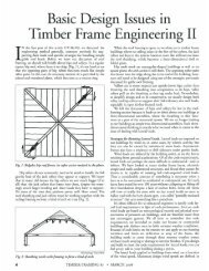
1.1. Timber Frame Introducti<strong>on</strong>/History<br />
Timber frames, c<strong>on</strong>sisting of heavy timber members with carpentry-style joinery,<br />
played an integral part in c<strong>on</strong>structi<strong>on</strong> for centuries, providing str<strong>on</strong>g <str<strong>on</strong>g>and</str<strong>on</strong>g> durable frames<br />
for structures of all kinds. Traditi<strong>on</strong>al timber framing utilizes several different types of<br />
joints for different c<strong>on</strong>necti<strong>on</strong> needs. Tensi<strong>on</strong> c<strong>on</strong>necti<strong>on</strong>s often use a mortise <str<strong>on</strong>g>and</str<strong>on</strong>g> ten<strong>on</strong><br />
joint (Figure 1-1); these joints use a wooden peg to fasten the ten<strong>on</strong> inside of the mortise.<br />
<strong>Mortise</strong><br />
Ten<strong>on</strong><br />
Post<br />
Beam<br />
Figure 1-1 <strong>Mortise</strong> <str<strong>on</strong>g>and</str<strong>on</strong>g> Ten<strong>on</strong> Joint from Schmidt <str<strong>on</strong>g>and</str<strong>on</strong>g> Daniels (1999)<br />
Increased producti<strong>on</strong> rates of saw mills <str<strong>on</strong>g>and</str<strong>on</strong>g> the ability to c<strong>on</strong>struct stick-frame<br />
structures in a short period of time lead to a shift in building methods away from of<br />
timber framing in the 19 th century. In recent decades however, timber framing has<br />
experienced a revival. With the revival in timber framing, new methods of enclosing the<br />
frame have been developed. Prefabricated panels can span between bays of the timber<br />
frame to provide a well insulated enclosure system. This development al<strong>on</strong>g with the<br />
1
ugged traditi<strong>on</strong>al style has helped lead to an ever increasing number of newly built <str<strong>on</strong>g>and</str<strong>on</strong>g><br />
restored traditi<strong>on</strong>al timber framed structures.<br />
1.2. Purpose/Need of Research<br />
In the past traditi<strong>on</strong>al timber frame joinery detailing was based <strong>on</strong> the craftsman’s<br />
experience. Currently specificati<strong>on</strong>s <str<strong>on</strong>g>and</str<strong>on</strong>g> detailing requirements for traditi<strong>on</strong>al timber<br />
frame joinery are not included in the Nati<strong>on</strong>al Design Specificati<strong>on</strong> (NDS) (AFPA, 1997)<br />
or in any other recognized code or design st<str<strong>on</strong>g>and</str<strong>on</strong>g>ard. Therefore values for strength <str<strong>on</strong>g>and</str<strong>on</strong>g><br />
stiffness of these joints are often not known. This produces a need for design equati<strong>on</strong>s<br />
<str<strong>on</strong>g>and</str<strong>on</strong>g> specificati<strong>on</strong>s that can be used to obtain the strength <str<strong>on</strong>g>and</str<strong>on</strong>g> stiffness of a mortise <str<strong>on</strong>g>and</str<strong>on</strong>g><br />
ten<strong>on</strong> joint.<br />
Tensi<strong>on</strong> strength of these joints is of primary interest, because it relies <strong>on</strong> the ability<br />
of the wood peg fasteners to carry the load. Tensi<strong>on</strong> can be developed in mortise <str<strong>on</strong>g>and</str<strong>on</strong>g><br />
ten<strong>on</strong> joints under both gravity <str<strong>on</strong>g>and</str<strong>on</strong>g> lateral loads. For instance, under gravity loads <strong>on</strong><br />
floor girders, knee braces carry compressi<strong>on</strong>, producing a lateral thrust <strong>on</strong> the posts. This<br />
thrust is resisted by a tensi<strong>on</strong> c<strong>on</strong>necti<strong>on</strong> between the girder <str<strong>on</strong>g>and</str<strong>on</strong>g> the post.<br />
The lateral load resistance of many timber-framed structures originates from a knee<br />
brace design. Knee braces are comm<strong>on</strong>ly seen in pairs. Under lateral load <strong>on</strong>e knee<br />
brace is in compressi<strong>on</strong> while the other is in tensi<strong>on</strong>. Examples of typical bents are<br />
shown below in Figure 1-2.<br />
2
Figure 1-2 Typical Bent Types from Schmidt <str<strong>on</strong>g>and</str<strong>on</strong>g> Daniels (1999)<br />
Often a timber frame designer has to over design a compressi<strong>on</strong> knee brace because<br />
of the uncertainty in strength <str<strong>on</strong>g>and</str<strong>on</strong>g> stiffness of a knee brace in tensi<strong>on</strong>. The compressi<strong>on</strong><br />
joint is over designed because the knee brace in tensi<strong>on</strong> is assumed have zero tensile<br />
capacity. The majority of timber frame knee brace c<strong>on</strong>necti<strong>on</strong>s are mortise <str<strong>on</strong>g>and</str<strong>on</strong>g> ten<strong>on</strong><br />
joints. A set of design st<str<strong>on</strong>g>and</str<strong>on</strong>g>ards would allow a timber frame designer to let the tensi<strong>on</strong><br />
brace carry a porti<strong>on</strong> of the lateral load.<br />
<str<strong>on</strong>g>Load</str<strong>on</strong>g> durati<strong>on</strong> <str<strong>on</strong>g>and</str<strong>on</strong>g> seas<strong>on</strong>ing effects are also of c<strong>on</strong>cern when designing a timber<br />
frame joint. Timber frames are frequently cut <str<strong>on</strong>g>and</str<strong>on</strong>g> assembled while timbers are still<br />
green. In most cases cost <str<strong>on</strong>g>and</str<strong>on</strong>g> schedule c<strong>on</strong>straints limit the amount of time that timbers<br />
can be seas<strong>on</strong>ed prior to cutting for a frame. This results in frames with high initial<br />
moisture c<strong>on</strong>tent. L<strong>on</strong>g term effects <strong>on</strong> joint strength <str<strong>on</strong>g>and</str<strong>on</strong>g> stiffness are of c<strong>on</strong>cern<br />
particularly when analyzing or designing for serviceability. These l<strong>on</strong>g-term effects <strong>on</strong><br />
traditi<strong>on</strong>al timber frame joinery are also bey<strong>on</strong>d the scope of current design<br />
specificati<strong>on</strong>s. This research addresses <str<strong>on</strong>g>and</str<strong>on</strong>g> c<strong>on</strong>siders the effects of load durati<strong>on</strong> <strong>on</strong><br />
strength, stiffness <str<strong>on</strong>g>and</str<strong>on</strong>g> detailing requirements of mortise <str<strong>on</strong>g>and</str<strong>on</strong>g> ten<strong>on</strong> joints<br />
3
1.3. Literature Review<br />
Previous research c<strong>on</strong>cerning mortise <str<strong>on</strong>g>and</str<strong>on</strong>g> ten<strong>on</strong> joint strength <str<strong>on</strong>g>and</str<strong>on</strong>g> stiffness included<br />
joint tests by Schmidt <str<strong>on</strong>g>and</str<strong>on</strong>g> Daniels (1999) who performed full-scale tests <strong>on</strong> mortise <str<strong>on</strong>g>and</str<strong>on</strong>g><br />
ten<strong>on</strong> joints of several different species of wood. Schmidt <str<strong>on</strong>g>and</str<strong>on</strong>g> Daniels (1999) tested<br />
several green or partially seas<strong>on</strong>ed joints to determine minimum end, edge <str<strong>on</strong>g>and</str<strong>on</strong>g> spacing<br />
distances in order to ensure a ductile peg failure of the joint. The minimum detailing<br />
requirements are then used al<strong>on</strong>g with the European Yield Model equati<strong>on</strong>s adapted by<br />
Schmidt <str<strong>on</strong>g>and</str<strong>on</strong>g> MacKay (1997) <str<strong>on</strong>g>and</str<strong>on</strong>g> Schmidt <str<strong>on</strong>g>and</str<strong>on</strong>g> Daniels (1999) to find a joint strength.<br />
Work at Michigan Technological University (Reid, 1997; S<str<strong>on</strong>g>and</str<strong>on</strong>g>berg et al, 2000) with<br />
simplified mortise <str<strong>on</strong>g>and</str<strong>on</strong>g> ten<strong>on</strong> joints has also shown be of value in modeling, testing <str<strong>on</strong>g>and</str<strong>on</strong>g><br />
defining strength <str<strong>on</strong>g>and</str<strong>on</strong>g> stiffness of mortise <str<strong>on</strong>g>and</str<strong>on</strong>g> ten<strong>on</strong> joints. This work with simplified<br />
mortise <str<strong>on</strong>g>and</str<strong>on</strong>g> ten<strong>on</strong> joints incorporated a single peg with three separate pieces of sawn<br />
lumber making up the rest of the joint, a single main member, representing the ten<strong>on</strong>, <str<strong>on</strong>g>and</str<strong>on</strong>g><br />
the mortise c<strong>on</strong>sisting of two side members.<br />
<str<strong>on</strong>g>Durati<strong>on</strong></str<strong>on</strong>g> of load effects are included in design of timber members through an<br />
adjustment factor based <strong>on</strong> the Madis<strong>on</strong> curve (Figure 1-3). This relati<strong>on</strong>ship between<br />
load durati<strong>on</strong> <str<strong>on</strong>g>and</str<strong>on</strong>g> member strength was developed by research at the Forest Products<br />
Laboratory (Breyer et al, 1999) using small clear specimens in bending. Nevertheless,<br />
the time effects are assumed to apply to c<strong>on</strong>necti<strong>on</strong> strength as well.<br />
4
Madis<strong>on</strong> Curve<br />
2.5<br />
2<br />
<str<strong>on</strong>g>Load</str<strong>on</strong>g> <str<strong>on</strong>g>Durati<strong>on</strong></str<strong>on</strong>g> Factor (C D )<br />
1.5<br />
1<br />
0.5<br />
0<br />
1 Sec<strong>on</strong>d 1 Hour 1 M<strong>on</strong>th 1 Year 100 Years<br />
Time<br />
Figure 1-3 Madis<strong>on</strong> Curve<br />
Research relevant to load durati<strong>on</strong> <str<strong>on</strong>g>and</str<strong>on</strong>g> seas<strong>on</strong>ing of mortise <str<strong>on</strong>g>and</str<strong>on</strong>g> ten<strong>on</strong> joinery is<br />
limited. Researchers at the Forest Products Laboratory (Wilkins<strong>on</strong>, 1988) investigated<br />
effects of load durati<strong>on</strong> <strong>on</strong> bolted c<strong>on</strong>necti<strong>on</strong>s. Sixty-four Douglas fir joints were<br />
evaluated; a ½ inch diameter steel bolt, h<str<strong>on</strong>g>and</str<strong>on</strong>g> tight, was used to secure the three pieces<br />
together. Each piece was loaded parallel to grain with an end distance of four inches.<br />
The center member was three inches wide <str<strong>on</strong>g>and</str<strong>on</strong>g> the two side members were each 1-1/2<br />
inches wide. The sixty-four joints were divided into four groups, c<strong>on</strong>sisting of sixteen<br />
joints per group. The first group, the c<strong>on</strong>trol group, was subjected to <strong>on</strong>ly short-term<br />
ramp load to failure with a c<strong>on</strong>stant rate of deflecti<strong>on</strong>. The sec<strong>on</strong>d, third <str<strong>on</strong>g>and</str<strong>on</strong>g> fourth<br />
groups were each subjected to a c<strong>on</strong>stant load for <strong>on</strong>e year at 85%, 60%, <str<strong>on</strong>g>and</str<strong>on</strong>g> 30% of the<br />
short term mean ultimate load. A few of the joints failed during the year of c<strong>on</strong>stant load.<br />
5
However these failures were away from the joint area <str<strong>on</strong>g>and</str<strong>on</strong>g> not related to the joint itself.<br />
The joints were then tested to failure in a similar fashi<strong>on</strong> as the first group. Each of the<br />
three groups subjected to the l<strong>on</strong>g-term load produced a higher mean load than the<br />
c<strong>on</strong>trol group. The group that was loaded to 30% of the short-term load had the highest<br />
average maximum load of the three loaded groups followed by the 85% <str<strong>on</strong>g>and</str<strong>on</strong>g> the 60%<br />
groups respectively. The reas<strong>on</strong> for this strength increase is not known or understood.<br />
The creep rate of the joints was also m<strong>on</strong>itored; the 30% <str<strong>on</strong>g>and</str<strong>on</strong>g> 60% groups approached a<br />
zero creep rate while creep in the 85% group decreased in rate, but creep was still<br />
occurring after <strong>on</strong>e year (Wilkins<strong>on</strong>, 1988).<br />
More recently, research has involved effects of load rate (Rosowsky <str<strong>on</strong>g>and</str<strong>on</strong>g> Reinhold,<br />
1999) <str<strong>on</strong>g>and</str<strong>on</strong>g> short-term durati<strong>on</strong> of load (Fridley <str<strong>on</strong>g>and</str<strong>on</strong>g> Rosowsky, 1998) <strong>on</strong> wood<br />
c<strong>on</strong>necti<strong>on</strong>s. In the former study, nailed <str<strong>on</strong>g>and</str<strong>on</strong>g> screwed c<strong>on</strong>necti<strong>on</strong> specimens were loaded<br />
at a rate from 0.1 to 1000 in/min. These tests revealed no obvious effects of load rate <strong>on</strong><br />
either lateral load or withdrawal resistance of the test specimens. In the latter study,<br />
nailed c<strong>on</strong>necti<strong>on</strong>s were loaded to15, 20, <str<strong>on</strong>g>and</str<strong>on</strong>g> 30% of their average strength for 25 days to<br />
study creep resp<strong>on</strong>se, <str<strong>on</strong>g>and</str<strong>on</strong>g> other specimens were loaded to 80, 90, <str<strong>on</strong>g>and</str<strong>on</strong>g> 95% of average<br />
static strength for 60 days to study effects <strong>on</strong> strength. Repeated loading at the latter high<br />
load levels was performed to study cyclic load effects. The creep <str<strong>on</strong>g>and</str<strong>on</strong>g> c<strong>on</strong>stant load<br />
specimens showed no ill effects of their load histories, whereas the cyclic load specimens<br />
did show reduced residual strength.<br />
No research <strong>on</strong> the seas<strong>on</strong>ing of mortise <str<strong>on</strong>g>and</str<strong>on</strong>g> ten<strong>on</strong> joints under load has been found.<br />
Often timber frame structures are c<strong>on</strong>structed with green timber <str<strong>on</strong>g>and</str<strong>on</strong>g> dried while in<br />
service c<strong>on</strong>diti<strong>on</strong>s. Therein lies the motivati<strong>on</strong> for this research.<br />
6
1.4. Objectives <str<strong>on</strong>g>and</str<strong>on</strong>g> Scope<br />
Three primary objectives exist for this research. The first is to determine effects of<br />
seas<strong>on</strong>ing <str<strong>on</strong>g>and</str<strong>on</strong>g> load durati<strong>on</strong> <strong>on</strong> traditi<strong>on</strong>al mortise <str<strong>on</strong>g>and</str<strong>on</strong>g> ten<strong>on</strong> joints under tensi<strong>on</strong>. To the<br />
extent possible, load durati<strong>on</strong> effects are separated from seas<strong>on</strong>ing effects <str<strong>on</strong>g>and</str<strong>on</strong>g> each is<br />
analyzed.<br />
The sec<strong>on</strong>d objective is to c<strong>on</strong>tinue the work of Schmidt <str<strong>on</strong>g>and</str<strong>on</strong>g> Daniels (1999). This<br />
research will c<strong>on</strong>tinue to develop end, edge <str<strong>on</strong>g>and</str<strong>on</strong>g> spacing distances for different species of<br />
wood. This phase of research will also serve in further development <str<strong>on</strong>g>and</str<strong>on</strong>g> validati<strong>on</strong> of a<br />
method in which dowel bearing strength <str<strong>on</strong>g>and</str<strong>on</strong>g> stiffness of a base material loaded with a<br />
wood peg fastener can be predicted mathematically. The advantages of mathematically<br />
predicting strength <str<strong>on</strong>g>and</str<strong>on</strong>g> stiffness could be of great value to future research by eliminating<br />
the need to perform combined material tests.<br />
The third objective is to use results from the l<strong>on</strong>g-term joint tests to c<strong>on</strong>firm or<br />
reassess detailing procedures for design of mortise <str<strong>on</strong>g>and</str<strong>on</strong>g> ten<strong>on</strong> joints. If appropriate a load<br />
durati<strong>on</strong> factor could then be defined for use in c<strong>on</strong>necti<strong>on</strong> design to adjust for load<br />
durati<strong>on</strong> effects <strong>on</strong> strength.<br />
The scope of the l<strong>on</strong>g-term research is inclusive of four different species of wood:<br />
southern yellow pine, Douglas fir, white oak, <str<strong>on</strong>g>and</str<strong>on</strong>g> eastern white pine. During the l<strong>on</strong>gterm<br />
load study, loading ranged from no load <strong>on</strong> specimens in the c<strong>on</strong>trol groups to<br />
sustained load of 1000 lb or 2000 lb <strong>on</strong> the remaining specimens. The magnitude of the<br />
l<strong>on</strong>g-term load is dependent up<strong>on</strong> the short-term strength of the joints.<br />
7
1.5. Overview<br />
Primary am<strong>on</strong>g the three objectives given above is to determine the effects of l<strong>on</strong>gterm<br />
loading <str<strong>on</strong>g>and</str<strong>on</strong>g> seas<strong>on</strong>ing <strong>on</strong> mortise <str<strong>on</strong>g>and</str<strong>on</strong>g> ten<strong>on</strong> joints in tensi<strong>on</strong>. In order to achieve<br />
this objective, tests <str<strong>on</strong>g>and</str<strong>on</strong>g> m<strong>on</strong>itoring of mortise <str<strong>on</strong>g>and</str<strong>on</strong>g> ten<strong>on</strong> joints were required. However,<br />
the first tests that were c<strong>on</strong>ducted involved short-term joint tests <strong>on</strong> eastern white pine<br />
joints; these tests were a c<strong>on</strong>tinuati<strong>on</strong> of the research c<strong>on</strong>ducted by Schmidt <str<strong>on</strong>g>and</str<strong>on</strong>g> Daniels<br />
(1999). These tests were needed to determine the minimum detailing requirements of the<br />
eastern white pine joints that were used in l<strong>on</strong>g-term tests.<br />
Following the short-term tests; joints of four different species were assembled. For<br />
each species, the joints were divided into a load group <str<strong>on</strong>g>and</str<strong>on</strong>g> a c<strong>on</strong>trol group. The c<strong>on</strong>trol<br />
group was not loaded <str<strong>on</strong>g>and</str<strong>on</strong>g> served as a basis for comparis<strong>on</strong> in later strength testing. Each<br />
of the remaining joints was subjected to a sustained load of 1000 lb or 2000 lb for a<br />
period of up to 348 days. Moisture c<strong>on</strong>tent was m<strong>on</strong>itored in <strong>on</strong>ly the c<strong>on</strong>trol group.<br />
<str<strong>on</strong>g>Effects</str<strong>on</strong>g> of drawboring <str<strong>on</strong>g>and</str<strong>on</strong>g> peg diameter were also compared using the time-deflecti<strong>on</strong><br />
plots produced from the l<strong>on</strong>g-term tests.<br />
Following the l<strong>on</strong>g-term tests, short-term load tests to failure were performed <strong>on</strong> all<br />
the joints. The yield values <str<strong>on</strong>g>and</str<strong>on</strong>g> stiffness of the loaded <str<strong>on</strong>g>and</str<strong>on</strong>g> unloaded groups were then<br />
compared. Additi<strong>on</strong>al factors such as peg diameter <str<strong>on</strong>g>and</str<strong>on</strong>g> effects of drawboring will also be<br />
analyzed. With the load durati<strong>on</strong> tests completed, minimum detailing requrements were<br />
then revisited with the load durati<strong>on</strong> tests completed <str<strong>on</strong>g>and</str<strong>on</strong>g> adjustments were made if<br />
needed.<br />
As a sec<strong>on</strong>dary objective a method of mathematically combining dowel bearing<br />
strength <str<strong>on</strong>g>and</str<strong>on</strong>g> stiffness was tested <str<strong>on</strong>g>and</str<strong>on</strong>g> verified. The material for this group of tests came<br />
8
from the short-term eastern white pine joint tests. Base material was tested both parallel<br />
<str<strong>on</strong>g>and</str<strong>on</strong>g> perpendicular to grain..<br />
In the next chapter, short-term tests of eastern white pine joints are described. These<br />
tests were performed to establish target strength values <str<strong>on</strong>g>and</str<strong>on</strong>g> detailing requirements for the<br />
joints used in the l<strong>on</strong>g-term study. Chapter 3 describes the method for determining the<br />
dowel bearing strength of wood with n<strong>on</strong>metalic (in this case, wood) fasteners. The timedependent<br />
behavior of pegged mortise <str<strong>on</strong>g>and</str<strong>on</strong>g> ten<strong>on</strong> joints under l<strong>on</strong>g-term load is presented<br />
in Chapter 4, <str<strong>on</strong>g>and</str<strong>on</strong>g> Chapter 5 c<strong>on</strong>tains the results of failure testing of the specimens<br />
subjected to l<strong>on</strong>g-term load. Analysis of the test results, plus a summary <str<strong>on</strong>g>and</str<strong>on</strong>g> c<strong>on</strong>clusi<strong>on</strong>s<br />
are presented in Chapter 6.<br />
9
2. Joint Tests (Eastern White Pine)<br />
2.1. Introducti<strong>on</strong><br />
Schmidt <str<strong>on</strong>g>and</str<strong>on</strong>g> Daniels (1999) reported joint detailing requirements al<strong>on</strong>g with tensi<strong>on</strong><br />
test results for three different species of wood. The reported results were from full-scale<br />
tests <strong>on</strong> southern yellow pine, recycled Douglas fir <str<strong>on</strong>g>and</str<strong>on</strong>g> red oak joints. In a c<strong>on</strong>tinuati<strong>on</strong><br />
of this work, tests of a similar nature were performed <strong>on</strong> eastern white pine joints.<br />
Detailing requirement are composed of end (l e ), edge (l v ) <str<strong>on</strong>g>and</str<strong>on</strong>g> spacing (l s ) distances.<br />
These distances are illustrated in Figure 2-1 below.<br />
l s<br />
l v<br />
e l<br />
Figure 2-1 Detailing Distances from Schmidt <str<strong>on</strong>g>and</str<strong>on</strong>g> Daniels (1999)<br />
Yielding of the peg is the preferred mode of joint failure. There are two primary<br />
reas<strong>on</strong>s for this. First, peg yielding leads to a ductile failure of the joint under tensi<strong>on</strong><br />
loading. The sec<strong>on</strong>d reas<strong>on</strong> is that the joint can be repaired by replacing the failed pegs<br />
with new <strong>on</strong>es. This mode of failure also helps to isolate the peg as the primary design<br />
criteri<strong>on</strong> of the joint. Alternate joint failure modes include mortise splitting <str<strong>on</strong>g>and</str<strong>on</strong>g> ten<strong>on</strong><br />
10
upture. Bearing failure of the peg, mortise or ten<strong>on</strong> could also c<strong>on</strong>trol the joint design,<br />
but such bearing failures have not been observed.<br />
2.2. Test Frame Set-up<br />
In order to find the minimum end, edge <str<strong>on</strong>g>and</str<strong>on</strong>g> spacing requirements, full-scale joint<br />
tests were performed <strong>on</strong> mortise <str<strong>on</strong>g>and</str<strong>on</strong>g> ten<strong>on</strong> joints c<strong>on</strong>structed from eastern white pine.<br />
The test frame was the same as was used in previous research (Schmidt <str<strong>on</strong>g>and</str<strong>on</strong>g> MacKay,<br />
1997). The test set up c<strong>on</strong>sists of an “A” frame with an Enerpac RCH 123 hydraulic ram,<br />
which applies a tensile force to the ten<strong>on</strong> member; see Figure 2-2. The base of the frame<br />
restrains moti<strong>on</strong> of the mortise piece. Two 2” linear potentiometers record joint<br />
displacement. The potentiometers are attached to the ten<strong>on</strong> member with the tip resting<br />
<strong>on</strong> the mortise member. Labview data acquisiti<strong>on</strong> software was used to record <str<strong>on</strong>g>and</str<strong>on</strong>g><br />
average the two potentiometer readings. Readings from a pressure transducer were<br />
recorded <str<strong>on</strong>g>and</str<strong>on</strong>g> combined with the potentiometer readings to plot load verses deflecti<strong>on</strong>.<br />
The load-deflecti<strong>on</strong> plot was used during the test to determine when the joint was<br />
yielding <str<strong>on</strong>g>and</str<strong>on</strong>g> when the test could be stopped.<br />
11
Figure 2-2 Short Term Test Set-up from Schmidt <str<strong>on</strong>g>and</str<strong>on</strong>g> MacKay (1997)<br />
2.3. Short Term Test Procedure<br />
The short term m<strong>on</strong>ot<strong>on</strong>ic test procedure was modeled after research c<strong>on</strong>ducted by<br />
Schmidt <str<strong>on</strong>g>and</str<strong>on</strong>g> Daniels (1999). Timber frame members for each joint were r<str<strong>on</strong>g>and</str<strong>on</strong>g>omly<br />
selected <str<strong>on</strong>g>and</str<strong>on</strong>g> checked for defects. The joint was lightly clamped together to assure a<br />
secure fit. Two peg holes were then drilled at a locati<strong>on</strong> that was thought to the minimum<br />
end <str<strong>on</strong>g>and</str<strong>on</strong>g> edge distance required to achieve peg failure. Two pegs were r<str<strong>on</strong>g>and</str<strong>on</strong>g>omly selected<br />
out of the same populati<strong>on</strong> used by Schmidt <str<strong>on</strong>g>and</str<strong>on</strong>g> Daniels for their joint tests. The pegs<br />
were oriented tangentially, with growth rings in the same directi<strong>on</strong> as applied force. The<br />
pegs were then driven with a mallet until secure.<br />
The joint was placed into the test frame <str<strong>on</strong>g>and</str<strong>on</strong>g> the two linear potentiometers were<br />
fastened to the ten<strong>on</strong> with wood screws. A troubleshooting Labview data acquisiti<strong>on</strong><br />
program was run to check for data acquisiti<strong>on</strong> errors. If no errors were detected, the<br />
program used for testing was started. Start time then was recorded <str<strong>on</strong>g>and</str<strong>on</strong>g> loading began.<br />
12
Pressure was applied to the hydraulic ram by way of a h<str<strong>on</strong>g>and</str<strong>on</strong>g> pump. A c<strong>on</strong>stant rate of<br />
deflecti<strong>on</strong> was maintained through the test. A deflecti<strong>on</strong> rate of 0.001 inches per sec<strong>on</strong>d<br />
was used. The test was c<strong>on</strong>tinued until the load deflecti<strong>on</strong> plot had clearly flattened or<br />
started to decline <str<strong>on</strong>g>and</str<strong>on</strong>g> a yield value using the 5% offset method could be established. The<br />
5% offset method of analysis will be discussed later in this chapter. After the joint<br />
yielded <str<strong>on</strong>g>and</str<strong>on</strong>g> had shown signs of failure, it was removed from the test frame. The pegs<br />
were then driven out <str<strong>on</strong>g>and</str<strong>on</strong>g> the joint was inspected. Observati<strong>on</strong>s about the test <str<strong>on</strong>g>and</str<strong>on</strong>g><br />
corresp<strong>on</strong>ding failure were then recorded.<br />
Dowel bearing tests followed the short-term joint tests. Two dowel bearing test<br />
samples were cut from each mortise member <str<strong>on</strong>g>and</str<strong>on</strong>g> two from each ten<strong>on</strong> member. Test<br />
results were recorded <str<strong>on</strong>g>and</str<strong>on</strong>g> moisture c<strong>on</strong>tent <str<strong>on</strong>g>and</str<strong>on</strong>g> specific gravity tests were also performed<br />
<strong>on</strong> the test samples.<br />
2.4. Failure Modes<br />
Joint failure is the result of failure in <strong>on</strong>e or more of the three joint comp<strong>on</strong>ents. The<br />
mortise member can split due to tensi<strong>on</strong> perpendicular to the grain (Figure 2-3). The split<br />
usually propagates from the peg holes <str<strong>on</strong>g>and</str<strong>on</strong>g> grows away from the joint parallel to the<br />
mortise member. This type failure of often occurs suddenly <str<strong>on</strong>g>and</str<strong>on</strong>g> without warning. It is a<br />
result of inadequate edge distance <strong>on</strong> the loaded edge of the member.<br />
13
Figure 2-3 Typical <strong>Mortise</strong> Member Failure from Schmidt <str<strong>on</strong>g>and</str<strong>on</strong>g> Daniels (1999)<br />
The ten<strong>on</strong> can fail (Figure 2-4); ten<strong>on</strong> failure is also referred to as a relish failure.<br />
The porti<strong>on</strong> of the ten<strong>on</strong> behind the peg holes can develop a single split, or a c<strong>on</strong>diti<strong>on</strong> of<br />
block shear failure is also comm<strong>on</strong>. Providing adequate end distance <strong>on</strong> the ten<strong>on</strong> can<br />
c<strong>on</strong>trol this failure mode.<br />
Figure 2-4 Typical Ten<strong>on</strong> Member Failure from Schmidt <str<strong>on</strong>g>and</str<strong>on</strong>g> Daniels (1999)<br />
Peg failure results in the most ductile failure mode. Typically two transverse failure<br />
planes form at the mortise-ten<strong>on</strong> interfaces as in Figure 2-5. The failure planes are<br />
formed from a combinati<strong>on</strong> of shear <str<strong>on</strong>g>and</str<strong>on</strong>g> bending stress. Peg failure of another type is<br />
also possible. A single plastic hinge can develop in the center of the ten<strong>on</strong>, shown in<br />
14
Figure 2-6. This type failure can develop in some c<strong>on</strong>necti<strong>on</strong>s with relatively large<br />
diameter pegs <str<strong>on</strong>g>and</str<strong>on</strong>g> thin ten<strong>on</strong>s. Failure of this type is comm<strong>on</strong> with base material of low<br />
dowel bearing strength.<br />
Figure 2-5 Peg Shear Bending Failure from Schmidt <str<strong>on</strong>g>and</str<strong>on</strong>g> Daniels (1999)<br />
P/2<br />
P<br />
P/2<br />
Figure 2-6 Peg Bending Failure Mode<br />
2.5. Analysis Methods (5% offset)<br />
A 5% offset method (ASTM D5764)(ASTM, 1999) was used to determine yield<br />
values in this research. The first step in this analysis method is to identify the initial<br />
linear porti<strong>on</strong> of the load deflecti<strong>on</strong> plot. The 5% offset method then uses an intercept<br />
line that is parallel to the linear porti<strong>on</strong> of the load deflecti<strong>on</strong> plot. This intercept line is<br />
15
offset horiz<strong>on</strong>tally a distance of 5% of the peg diameter of the test in questi<strong>on</strong>. The<br />
intersecti<strong>on</strong> of the load deflecti<strong>on</strong> line <str<strong>on</strong>g>and</str<strong>on</strong>g> the 5% offset intercept line is then taken as the<br />
yield value. If a higher value for load is observed before the intercept, then that higher<br />
value will become the yield value. Figure 2-7 shows a typical load deflecti<strong>on</strong> curve <str<strong>on</strong>g>and</str<strong>on</strong>g><br />
the yield value found from that curve using the 5% offset method for determining yield<br />
value. A spreadsheet program was created <str<strong>on</strong>g>and</str<strong>on</strong>g> used to automate this process for this<br />
research.<br />
<str<strong>on</strong>g>Load</str<strong>on</strong>g> vs Deflecti<strong>on</strong><br />
12000<br />
10000<br />
10744<br />
<str<strong>on</strong>g>Load</str<strong>on</strong>g> (lbs)<br />
8000<br />
6000<br />
4000<br />
0.05D<br />
2000<br />
0<br />
0.00 0.05 0.10 0.15<br />
Deflecti<strong>on</strong> (In)<br />
Figure 2-7 5% Offset Yield Value Example<br />
2.6. Results<br />
Nine eastern white pine joints were fabricated <str<strong>on</strong>g>and</str<strong>on</strong>g> tested with white oak pegs.<br />
Bensen Woodworking of Alstead Center New Hampshire d<strong>on</strong>ated the joints. Pegs were<br />
taken from the same sample group that Schmidt <str<strong>on</strong>g>and</str<strong>on</strong>g> Daniels (1999) used for their joint<br />
16
tests. End <str<strong>on</strong>g>and</str<strong>on</strong>g> edge distance was varied to achieve a minimum distance <str<strong>on</strong>g>and</str<strong>on</strong>g> still achieve<br />
ductile peg failure. Peg spacing was c<strong>on</strong>stant at three inches. If a joint was tested <str<strong>on</strong>g>and</str<strong>on</strong>g><br />
<strong>on</strong>ly the pegs failed, a repair was made by replacing the pegs. The joint was then tested<br />
again <str<strong>on</strong>g>and</str<strong>on</strong>g> is denoted by a B following the test joint number. A summary of the eastern<br />
white pine joint tests follows in Table 2-1.<br />
Table 2-1 Eastern White Pine Joint Test Summary<br />
Peg<br />
Diameter End Dist. Edge Spacing Yield<br />
Yield<br />
<str<strong>on</strong>g>Load</str<strong>on</strong>g> Stiffness Ult. Disp Ult. <str<strong>on</strong>g>Load</str<strong>on</strong>g> Ave.<br />
Failure<br />
Type @<br />
Failure<br />
Type @<br />
Test (in) (D) Dist. (D) Dist. (D) Disp. (in) (lbs) (lbs/in) (in) (lbs) Peg G Yield Ultimate<br />
EWP 01 1 2.5 2.5 3 0.13 4720 55,900 0.27 5160 0.649 <strong>Mortise</strong>/Peg <strong>Mortise</strong>/Peg<br />
EWP 02 1 2.5 2.5 3 0.22 5010 31,300 0.26 5370 0.451 Ten<strong>on</strong>/Peg Ten<strong>on</strong>/Peg<br />
EWP 03 1 3 3 3 0.17 5160 40,200 0.24 5870 0.842 <strong>Mortise</strong>/Peg <strong>Mortise</strong>/Peg<br />
EWP 04 0.75 4 4 4 0.11 2540 28,400 0.32 3520 0.668 Peg Peg<br />
EWP 04B 0.75 4 4 4 0.19 3320 18,100 0.32 3580 0.718 Peg Peg<br />
EWP 05 0.75 3 3 4 0.10 2400 34,000 0.31 3350 0.719 Peg Peg<br />
EWP 06 0.75 3 3 4 0.08 2570 54,700 0.25 3340 0.762 Ten<strong>on</strong> Ten<strong>on</strong><br />
EWP 07 0.75 4 4 4 0.13 3530 30,100 0.25 3860 0.675 Peg <strong>Mortise</strong><br />
EWP 08 1 4 4 3 0.15 5790 53,900 0.18 5920 0.652 Peg Peg<br />
EWP 08B 1 4 4 3 0.21 6750 41,900 0.25 7090 0.813 Peg <strong>Mortise</strong><br />
EWP 09 0.75 4 4 4 0.14 3090 25,700 0.23 3480 0.612 Peg <strong>Mortise</strong>/Peg<br />
Mean 3/4" 2910 31,830<br />
Mean 1" 5490 44,640<br />
The relatively small number of joints tested <str<strong>on</strong>g>and</str<strong>on</strong>g> the different peg diameters make<br />
statistical work, such as determining a lower 5% exclusi<strong>on</strong> limit <strong>on</strong> strength, to be of<br />
questi<strong>on</strong>able value. Mean stiffness <str<strong>on</strong>g>and</str<strong>on</strong>g> yield values are reported in Table 2-1 as a<br />
functi<strong>on</strong> of peg diameter. Minimum detailing requirements for end <str<strong>on</strong>g>and</str<strong>on</strong>g> edge distances<br />
were found. Spacing distance (l s ) was c<strong>on</strong>sidered to be an issue of c<strong>on</strong>structi<strong>on</strong> detailing<br />
according to Schmidt <str<strong>on</strong>g>and</str<strong>on</strong>g> Daniels (1999). Minimum end (l e ) <str<strong>on</strong>g>and</str<strong>on</strong>g> edge (l v ) distances were<br />
found to be 4 peg diameters for eastern white pine (see Figure 2-1).<br />
This distance is somewhat larger than the end <str<strong>on</strong>g>and</str<strong>on</strong>g> edge distances that Schmidt <str<strong>on</strong>g>and</str<strong>on</strong>g><br />
Daniels (1999) reported. However, the strength <str<strong>on</strong>g>and</str<strong>on</strong>g> specific gravity of the eastern white<br />
pine is lower than that of the species they tested.<br />
17
2.7. Dowel Bearing Strength<br />
Dowel bearing tests were c<strong>on</strong>ducted following the joint tests. Testing procedures of<br />
Schmidt <str<strong>on</strong>g>and</str<strong>on</strong>g> Daniels were followed. Two 4”x 4”x 1-1/2” blocks were cut from each<br />
mortise member <str<strong>on</strong>g>and</str<strong>on</strong>g> each ten<strong>on</strong> member. The samples were knot <str<strong>on</strong>g>and</str<strong>on</strong>g> check free if<br />
possible. The samples were orientated in the directi<strong>on</strong> they would be in the joint. The<br />
mortise member samples were loaded perpendicular to grain <str<strong>on</strong>g>and</str<strong>on</strong>g> tensi<strong>on</strong> member<br />
samples were loaded parallel to grain. The 5% offset method of analysis was used. All<br />
the dowel bearing samples were tested with a <strong>on</strong>e-inch diameter steel rod. A time delay<br />
occured between the joint tests <str<strong>on</strong>g>and</str<strong>on</strong>g> cutting of dowel bearing specimens. This delay<br />
resulted in a loss of moisture c<strong>on</strong>tent in the material. Additi<strong>on</strong>al specimens were cut for<br />
the purpose of verifying a spring theory that will be discussed later in Chapter 3. A<br />
summary of the dowel bearing results is provided in Table 2-2. In the table, the value K<br />
is the number of st<str<strong>on</strong>g>and</str<strong>on</strong>g>ard deviati<strong>on</strong>s between the mean yield value <str<strong>on</strong>g>and</str<strong>on</strong>g> the lower 5%<br />
exclusi<strong>on</strong> limit, using a 75% c<strong>on</strong>fidence level (see Table 3, ASTM D 2915).<br />
18
Table 2-2 Eastern White Pine Dowel Bearing Test Results<br />
Number Yield Value (lbs/in 2 ) Stiffness (lbs/in 3 ) Number Yield Value (lbs/in 2 ) Stiffness (lbs/in 3 )<br />
EWP01M1 1,950 20,300 EWP01T1 4,890 115,300<br />
EWP01M2 1,720 16,000 EWP01T2 4,590 118,200<br />
EWP02M1 1,640 16,600 EWP02T1 4,960 120,300<br />
EWP02M2 1,420 12,900 EWP02T2 4,660 98,300<br />
EWP03M1 1,530 12,900 EWP03T1 4,800 86,400<br />
EWP03M2 1,490 14,500 EWP03T2 4,570 92,100<br />
EWP04M1 1,800 16,200 EWP04T1 5,830 137,500<br />
EWP04M2 1,960 23,300 EWP04T2 5,560 140,600<br />
EWP05M1 1,390 12,100 EWP05T1 5,270 120,500<br />
EWP05M2 1,730 15,600 EWP05T2 6,100 162,000<br />
EWP06M1 1,680 17,500 EWP06T1 5,140 160,400<br />
EWP06M2 1,720 17,800 EWP06T2 4,580 105,900<br />
EWP07M1 2,000 28,600 EWP07T1 3,840 96,000<br />
EWP07M2 2,950 27,100 EWP07T2 3,940 87,100<br />
EWP08M1 1,490 13,100 EWP08T1 4,390 98,200<br />
EWP08M2 1,640 14,500 EWP08T2 4,100 118,900<br />
Mean 1,760 17,400 Mean 4,830 116,100<br />
St. Dev. 370 5,000 St. Dev. 640 24,000<br />
5% Exclusi<strong>on</strong> 1,030 5% Exclusi<strong>on</strong> 3,560<br />
COV 0.210 COV 0.133<br />
K 1.977 K 1.977<br />
Dowel bearing test results are reported in a different way than in previous research.<br />
The procedure used to report bearing stiffness in this research was to divide the initial<br />
slope of the load deflecti<strong>on</strong> plot by the specimen width <str<strong>on</strong>g>and</str<strong>on</strong>g> the peg diameter. The yield<br />
load of the sample has been c<strong>on</strong>verted to a yield stress. Yield stress has also been found<br />
using the width of the specimen <str<strong>on</strong>g>and</str<strong>on</strong>g> the peg diameter, similar to past procedures used by<br />
Schmidt <str<strong>on</strong>g>and</str<strong>on</strong>g> MacKay (1997) <str<strong>on</strong>g>and</str<strong>on</strong>g> Schmidt <str<strong>on</strong>g>and</str<strong>on</strong>g> Daniels (1999).<br />
The stiffness calculati<strong>on</strong>s of previous research did not take into account the exact<br />
width of the specimen, introducing the potential for error. The width of the specimen is<br />
directly related to the stiffness of the sample. A soluti<strong>on</strong> to this discrepancy is to report<br />
the stiffness in units of lbs/in 3 . The change in reporting stiffness values will lead to more<br />
accurate comparis<strong>on</strong>s between tests.<br />
19
2.8. Detailing Requirements (End/Edge/Spacing)<br />
Required end <str<strong>on</strong>g>and</str<strong>on</strong>g> edge distances for eastern white pine joints <str<strong>on</strong>g>and</str<strong>on</strong>g> the joint species<br />
that were tested by Schmidt <str<strong>on</strong>g>and</str<strong>on</strong>g> Daniels (1999) are summarized in Table 2-3. These<br />
detailing requirements resulted in peg failures using the 5% offset method of yield<br />
analysis. All of the joints tested to obtain these distances were unseas<strong>on</strong>ed <str<strong>on</strong>g>and</str<strong>on</strong>g> subjected<br />
to short term loading; failure was reached in approximately 10 to 15 minutes. L<strong>on</strong>g-term<br />
loading <str<strong>on</strong>g>and</str<strong>on</strong>g> seas<strong>on</strong>ing effects were not taken into c<strong>on</strong>siderati<strong>on</strong> when determining these<br />
minimum detailing requirements. A factor of safety is also not c<strong>on</strong>sidered in these<br />
calculati<strong>on</strong>s. However a factor of safety will not be applied in this area of design, but<br />
rather it will be incorporated into the design load of the joint.<br />
Table 2-3 Minimum Detailing Requirements (Used for l<strong>on</strong>g-term tests)<br />
Species End (D) Edge (D) Spacing (D)<br />
Douglas Fir 2 2.5 2.5<br />
Eastern White Pine 4 4 3*<br />
Red/White Oak 2 2 2.5<br />
Southern Yellow Pine 2** 2 3<br />
*A c<strong>on</strong>stant value of 3" was used for testing<br />
**3D with drawbore<br />
2.9. Joint Strength Correlati<strong>on</strong><br />
A correlati<strong>on</strong> between joint strength <str<strong>on</strong>g>and</str<strong>on</strong>g> the specific gravity of the joint material was<br />
examined. The joints in the correlati<strong>on</strong> study c<strong>on</strong>sisted of the recycled Douglas fir, red<br />
oak <str<strong>on</strong>g>and</str<strong>on</strong>g> southern pine joints tested by Schmidt <str<strong>on</strong>g>and</str<strong>on</strong>g> Daniels (1999), plus the eastern white<br />
pine joints tested in this research. All of the pegs in this study came from the same<br />
sample group of white oak. The yield stress for peg shear was then found as the average<br />
value <strong>on</strong> the peg cross secti<strong>on</strong>, using the yield load <str<strong>on</strong>g>and</str<strong>on</strong>g> assuming four shear planes, two<br />
20
shear planes per peg. This type of peg failure is the most comm<strong>on</strong> throughout all of the<br />
joints tested. Comparing shear stress rather than joint yield load also makes it possible to<br />
include results for the joints that were tested with 3/4” diameter pegs. A plot of the<br />
average shear yield stress versus base material specific gravity is shown in Figure 2-8.<br />
2500<br />
τ = 1617G + 1063<br />
R2 = 0.4638<br />
2000<br />
Mean Shear Stress at Yield<br />
1500<br />
1000<br />
500<br />
Red Oak<br />
Douglas Fir<br />
Souterh Yellow Pine<br />
Eastern White Pine<br />
0<br />
0 0.1 0.2 0.3 0.4 0.5 0.6 0.7 0.8<br />
Base Material Specific Gravity<br />
Figure 2-8 Correlati<strong>on</strong> of Specific Gravity to Peg Joint Shear Stress<br />
The base material specific gravity is related to base material strength. With a<br />
relati<strong>on</strong>ship between base material specific gravity <str<strong>on</strong>g>and</str<strong>on</strong>g> base material strength, a<br />
correlati<strong>on</strong> between c<strong>on</strong>finement strength <str<strong>on</strong>g>and</str<strong>on</strong>g> specific gravity is assumed. In other words<br />
a higher base material specific gravity equates to a larger peg shear yield value <str<strong>on</strong>g>and</str<strong>on</strong>g><br />
higher joint yield strength. With increased c<strong>on</strong>finement strength the peg is subjected to a<br />
smaller shear span L (Figure 2-9) over which it can deform producing a higher joint yield<br />
value.<br />
21
Figure 2-9 Illustrati<strong>on</strong> of Peg Failure<br />
22
3. Spring Theory<br />
3.1. Theory/Possible Uses<br />
Currently dowel bearing strength <str<strong>on</strong>g>and</str<strong>on</strong>g> stiffness for different species combinati<strong>on</strong>s of<br />
base <str<strong>on</strong>g>and</str<strong>on</strong>g> peg material can be found <strong>on</strong>ly by testing each base material species with the<br />
corresp<strong>on</strong>ding peg species. Obviously many tests would have to be performed in order to<br />
obtain a comprehensive table of strengths <str<strong>on</strong>g>and</str<strong>on</strong>g> stiffnesses for varying combinati<strong>on</strong>s of<br />
base <str<strong>on</strong>g>and</str<strong>on</strong>g> peg species. One possible soluti<strong>on</strong> would be to test the peg material <str<strong>on</strong>g>and</str<strong>on</strong>g> base<br />
material separately <str<strong>on</strong>g>and</str<strong>on</strong>g> then add the properties mathematically. The behavior of the<br />
combined materials is based <strong>on</strong> the theory that the two comp<strong>on</strong>ents of the joint, the base<br />
material <str<strong>on</strong>g>and</str<strong>on</strong>g> the peg, carry load as two springs in series. Figure 3-1 is a visual<br />
representati<strong>on</strong> of the spring theory.<br />
Steel<br />
Steel Rod<br />
Wood Peg<br />
+<br />
=<br />
Wood Peg<br />
Wood Base<br />
Wood Base<br />
Figure 3-1 Spring Theory C<strong>on</strong>cept from Schmidt <str<strong>on</strong>g>and</str<strong>on</strong>g> Daniels (1999)<br />
A procedure to combine the material data mathematically would reduce the need for<br />
future testing <str<strong>on</strong>g>and</str<strong>on</strong>g> make better use of the data that has already been acquired. This<br />
method of mathematically combining material properties is limited to the dowel bearing<br />
23
properties of a base material loaded with a wood peg. Schmidt <str<strong>on</strong>g>and</str<strong>on</strong>g> Daniels (1999)<br />
developed the theory. It is verified in this research.<br />
3.2. Test Procedures<br />
The species used were eastern white pine for the base material <str<strong>on</strong>g>and</str<strong>on</strong>g> white oak for the<br />
pegs. Test procedures were modeled after those performed by Schmidt <str<strong>on</strong>g>and</str<strong>on</strong>g> Daniels<br />
(1999). Three types of tests were needed in an effort to validate the spring theory. The<br />
first test is a dowel bearing test of the eastern white pine base material. The dowel<br />
bearing tests c<strong>on</strong>formed to ASTM D5764 with a stroke rate of 0.024 in/min (ASTM<br />
1999). (This stroke rate was increased to .050 in/min in some cases for the dowel bearing<br />
strengths of the l<strong>on</strong>g-term joints, reported in the appendices). The dowel bearing strength<br />
of the eastern white pine is found using a 4”x 4”x 1-1/2” specimen with a half circle 1” in<br />
diameter in the top (see Figure 3-2 below). A steel dowel is placed in the 1” diameter<br />
trough; load is then applied to the steel dowel.<br />
24
Figure 3-2 Base Material Dowel Bearing Test (From Schmidt <str<strong>on</strong>g>and</str<strong>on</strong>g> Daniels 1999)<br />
A peg bearing test is the sec<strong>on</strong>d type of test used. A peg bearing test uses a 1-1/2”<br />
square steel load block with a 1” diameter half circle in <strong>on</strong>e face. The peg is placed into a<br />
l<strong>on</strong>g shallow trough cut into a steel base plate with the ends of the peg clamped to the<br />
base plate to hold the peg flat during the test. The load block is placed <strong>on</strong> top of the peg.<br />
<str<strong>on</strong>g>Load</str<strong>on</strong>g> is applied to the load block to test the peg bearing strength (see Figure 3-3 below).<br />
Figure 3-3 Peg Dowel Bearing Test (From Schmidt <str<strong>on</strong>g>and</str<strong>on</strong>g> Daniels 1999)<br />
The third test involves a combinati<strong>on</strong> of the eastern white pine base material block<br />
<str<strong>on</strong>g>and</str<strong>on</strong>g> a white oak peg. The peg is secured in the trough of the base plate as in Figure 3-3,<br />
25
ut the load is applied through the base material block. The shallow trough prevents<br />
bearing failure of the peg remote from the interface between the peg <str<strong>on</strong>g>and</str<strong>on</strong>g> the base<br />
material. The test is similar to that shown in Figure 3-3 with the base material in place of<br />
the steel load block.<br />
3.3. Method <str<strong>on</strong>g>and</str<strong>on</strong>g> Results<br />
<str<strong>on</strong>g>Load</str<strong>on</strong>g>-deflecti<strong>on</strong> results of base material bearing <str<strong>on</strong>g>and</str<strong>on</strong>g> peg bearing tests were processed<br />
by a program that performed a filtering operati<strong>on</strong> <strong>on</strong> the load-displacement curve. The<br />
program smoothed the test data into uniform load increments of 25 pounds <str<strong>on</strong>g>and</str<strong>on</strong>g> found the<br />
corresp<strong>on</strong>ding displacement. The displacements of the two tests at the same load were<br />
then added in order to synthesize a load-displacement curve for the combined materials.<br />
The 5% offset method with a 1” peg diameter was <strong>on</strong>ce again used for all of the tests in<br />
questi<strong>on</strong>.<br />
In order to reduce variability <str<strong>on</strong>g>and</str<strong>on</strong>g> to achieve a higher degree of c<strong>on</strong>fidence, matched<br />
bearing samples were cut from each piece of eastern white pine. Four bearing samples<br />
were cut from each ten<strong>on</strong> member <str<strong>on</strong>g>and</str<strong>on</strong>g> each mortise member. Two of the four samples<br />
were used for the c<strong>on</strong>venti<strong>on</strong>al dowel bearing tests (Figure 3-2) <str<strong>on</strong>g>and</str<strong>on</strong>g> two for combined<br />
tests. To obtain matched specimens for the pegs, two-foot l<strong>on</strong>g pegs were cut in half so<br />
that <strong>on</strong>e half of the peg could be used in the peg bearing test (Figure 3-3) <str<strong>on</strong>g>and</str<strong>on</strong>g> the other<br />
half in the combined test. A test specimen distributi<strong>on</strong> table is given in Table 3-1.<br />
26
Table 3-1 Spring Theory Test Distributi<strong>on</strong><br />
Base Material Bearing Tests Peg Bearing Tests<br />
Mathematically Combined<br />
Physically Combined<br />
Ten<strong>on</strong> 1, Test 1 Peg 1 = Ten<strong>on</strong> 1 Average + Peg 1 Ten<strong>on</strong> 1 with Peg 1<br />
Ten<strong>on</strong> 1 Average +<br />
Ten<strong>on</strong> 1, Test 2 Peg 2 = Ten<strong>on</strong> 1 Average + Peg 2 Ten<strong>on</strong> 1 with Peg 2<br />
Ten<strong>on</strong> 2, Test 1 Peg 3 = Ten<strong>on</strong> 2 Average + Peg 3 Ten<strong>on</strong> 2 with Peg 3<br />
Ten<strong>on</strong> 2 Average +<br />
Ten<strong>on</strong> 2, Test 2 Peg 4 = Ten<strong>on</strong> 2 Average + Peg 4 Ten<strong>on</strong> 2 with Peg 4<br />
In total thirty-two comparis<strong>on</strong>s were made. Sixteen comparis<strong>on</strong>s were made from<br />
material taken from the mortise <str<strong>on</strong>g>and</str<strong>on</strong>g> sixteen comparis<strong>on</strong>s were made from material taken<br />
from the ten<strong>on</strong>. <strong>Mortise</strong> material was loaded perpendicular to the grain while the ten<strong>on</strong><br />
material was loaded parallel to the grain. As expected the difference in grain directi<strong>on</strong><br />
has a substantial effect <strong>on</strong> both the strength <str<strong>on</strong>g>and</str<strong>on</strong>g> stiffness of the material. The two-foot<br />
pegs were chosen r<str<strong>on</strong>g>and</str<strong>on</strong>g>omly from a separate supply; they were not from the sample group<br />
used for virtually every other peg from both this research <str<strong>on</strong>g>and</str<strong>on</strong>g> the research of Schmidt <str<strong>on</strong>g>and</str<strong>on</strong>g><br />
Daniels (1999). The pegs from that sample group were <strong>on</strong>e-foot l<strong>on</strong>g, making it<br />
impossible to achieve matched peg specimens for the study. Table 3-2 is a summary of<br />
results of the comparis<strong>on</strong>.<br />
27
Table 3-2 Spring Theory Summary<br />
Test<br />
Mathematically Combined Physically Combined Ratio (Mathematically/Physically)<br />
Number Yield Stress (lbs/in 2 ) Stiffness (lbs/in 3 ) Yield Stress (lbs/in 2 ) Stiffness (lbs/in 3 ) Yield Stress Stiffness<br />
M01 1,820 12,900 1,760 15,900 1.04 0.81<br />
M02 1,810 13,900 1,870 16,000 0.97 0.87<br />
M03 1,520 11,600 1,420 10,700 1.07 1.08<br />
M04 1,530 10,400 1,350 10,400 1.13 1.00<br />
M05 1,520 11,400 1,480 11,900 1.03 0.96<br />
M06 1,530 10,400 1,390 9,700 1.10 1.07<br />
M07 1,630 13,500 1,460 13,700 1.12 0.99<br />
M08 1,750 15,200 1,690 16,000 1.03 0.95<br />
M09 1,490 9,900 1,460 12,300 1.03 0.80<br />
M10 1,490 10,100 1,440 10,900 1.04 0.92<br />
M11 1,720 13,400 1,580 13,200 1.09 1.02<br />
M12 1,740 13,600 1,540 12,900 1.12 1.05<br />
M13 2,030 17,700 1,960 29,500 1.03 0.60<br />
M14 2,160 18,900 2,160 26,100 1.00 0.72<br />
M15 1,630 10,500 1,540 13,200 1.06 0.79<br />
M16 1,630 10,400 1,510 11,600 1.08 0.90<br />
Mean 1.06 0.91<br />
St<str<strong>on</strong>g>and</str<strong>on</strong>g>ard Deviati<strong>on</strong> 0.047 0.135<br />
Test<br />
Mathematically Combined Physically Combined Ratio (Mathematically/Physically)<br />
Number Yield Stress (lbs/in 2 ) Stiffness (lbs/in 3 ) Yield Stress (lbs/in 2 ) Stiffness (lbs/in 3 ) Yield Stress Stiffness<br />
T01 3,530 46,320 3,060 57,590 1.15 0.80<br />
T02 2,630 46,350 2,660 45,310 0.99 1.02<br />
T03 2,300 41,310 2,280 30,370 1.01 1.36<br />
T04 3,200 48,710 3,370 48,360 0.95 1.01<br />
T05 3,050 46,830 3,450 34,000 0.88 1.38<br />
T06 2,850 42,700 2,570 34,870 1.11 1.22<br />
T07 3,300 49,420 3,190 44,990 1.03 1.10<br />
T08 3,130 45,170 2,670 43,610 1.17 1.04<br />
T09 2,980 44,940 2,620 46,250 1.13 0.97<br />
T10 2,910 45,220 2,520 47,140 1.15 0.96<br />
T11 4,150 57,860 3,240 46,130 1.28 1.25<br />
T12 3,420 43,820 3,200 51,820 1.07 0.85<br />
T13 3,410 50,560 3,340 45,130 1.02 1.12<br />
T14 2,330 41,380 2,330 42,300 1.00 0.98<br />
T15 2,560 43,860 2,650 36,850 0.97 1.19<br />
T16 2,750 47,690 2,330 45,640 1.18 1.04<br />
Mean 1.07 1.08<br />
St<str<strong>on</strong>g>and</str<strong>on</strong>g>ard Deviati<strong>on</strong> 0.105 0.166<br />
In order to compare the strengths <str<strong>on</strong>g>and</str<strong>on</strong>g> stiffnesses of the tests, the mathematically<br />
combined results were divided by the physically combined results. A ratio of 1.00 would<br />
therefore corresp<strong>on</strong>d to the mathematical model perfectly representing the physically<br />
model. The 5% offset method of analysis was used to find results for both the<br />
mathematically combined <str<strong>on</strong>g>and</str<strong>on</strong>g> physically combined tests.<br />
Based <strong>on</strong> examinati<strong>on</strong> of the table, it is evident that the spring theory represents the<br />
combined material tests relatively well, given the natural variability of wood. In general<br />
the spring theory showed a higher value for strength. With unity values ranging between<br />
0.88 <str<strong>on</strong>g>and</str<strong>on</strong>g> 1.28, the spring theory accurately predicted the combined material test yield<br />
values.<br />
28
The difference in stiffness values was also within a reas<strong>on</strong>able range. Unity values<br />
varied between 0.60 <str<strong>on</strong>g>and</str<strong>on</strong>g> 1.28 with an average perpendicular to grain ratio of 0.91 <str<strong>on</strong>g>and</str<strong>on</strong>g> an<br />
average parallel to grain ratio of 1.08. In general the mathematically combined tests<br />
represented the physically combined tests well.<br />
The eastern white pine base material has a significantly lower bearing strength<br />
perpendicular to grain than the white oak used for the pegs (see Figure 3-4). The<br />
difference in bearing strength meant that the weaker eastern white pine material<br />
dominated the test results; often in the combined tests, little peg damage was visible.<br />
While difficult to quantify, this effect is a c<strong>on</strong>siderati<strong>on</strong>.<br />
<str<strong>on</strong>g>Load</str<strong>on</strong>g> (lbs)<br />
5000<br />
4000<br />
3000<br />
2000<br />
1000<br />
Peg Bearing Test<br />
Dowel Bearing Test <strong>on</strong><br />
Base Material<br />
Mathematically Combined Test<br />
Linear Porti<strong>on</strong> of Physically<br />
Combined Test<br />
Linear Porti<strong>on</strong> of<br />
Mathematically<br />
Combined Test<br />
Physically Combined Test<br />
0<br />
0.000 0.050 0.100 0.150 0.200 0.250 0.300 0.350<br />
Deflecti<strong>on</strong> (in)<br />
Figure 3-4 Typical Spring Theory Plot (Base Material <str<strong>on</strong>g>Load</str<strong>on</strong>g>ed Perpendicular to Grain)<br />
Combined tests with the base material loaded parallel to grain resulted in more peg<br />
damage. In the tests with the base material loaded parallel to grain the base material was<br />
29
the stiffer of the two materials; resulting in the peg material properties dominating the<br />
combined tests (see Figure 3-5).<br />
8000<br />
6000<br />
Dowel Bearing Test<br />
<strong>on</strong> Base Material<br />
Linear Porti<strong>on</strong><br />
of Physically<br />
Combined Test<br />
Linear of<br />
Mathematically<br />
Combined Test<br />
Peg Bearing Test<br />
<str<strong>on</strong>g>Load</str<strong>on</strong>g> (lbs)<br />
4000<br />
2000<br />
Physically Combined Test<br />
Mathematically Combined<br />
0<br />
0.000 0.050 0.100 0.150 0.200 0.250<br />
Deflecti<strong>on</strong> (in)<br />
Figure 3-5 Typical Spring Theory Plot (Base Material <str<strong>on</strong>g>Load</str<strong>on</strong>g>ed Parallel to Grain)<br />
With the material of lower strength <str<strong>on</strong>g>and</str<strong>on</strong>g> stiffness dominating the combined test<br />
results, a comparis<strong>on</strong> of the combined test results verses the test results of <strong>on</strong>ly the<br />
weaker/softer material was performed. Table 3-3 below is a comparis<strong>on</strong> of the<br />
properties of the weaker/softer material versus the combined test results. The<br />
weaker/softer material being the base material when loaded perpendicular to grain <str<strong>on</strong>g>and</str<strong>on</strong>g><br />
the peg when the base material is loaded parallel to grain (see Figure 3-4 <str<strong>on</strong>g>and</str<strong>on</strong>g> Figure 3-5).<br />
30
Table 3-3 Comparis<strong>on</strong> of Combined Test Results with Weaker/Softer Material<br />
Test<br />
Mathematically Combined<br />
Physically Combined<br />
Difference (Mathematically/Physically)<br />
Number Yield Stress (lbs/in 2 ) Stiffness (lbs/in 3 ) Yield Stress (lbs/in 2 ) Stiffness (lbs/in 3 ) Yield Stress Stiffness<br />
M01 1,760 15,900 1,840 18,200 0.96 0.87<br />
M02 1,870 16,000 1,840 18,200 1.02 0.88<br />
M03 1,420 10,700 1,530 14,700 0.93 0.73<br />
M04 1,350 10,400 1,530 14,700 0.88 0.71<br />
M05 1,480 11,900 1,510 13,700 0.98 0.87<br />
M06 1,390 9,700 1,510 13,700 0.92 0.71<br />
M07 1,460 13,700 1,880 19,700 0.78 0.70<br />
M08 1,690 16,000 1,880 19,700 0.90 0.81<br />
M09 1,460 12,300 1,560 13,800 0.94 0.89<br />
M10 1,440 10,900 1,560 13,800 0.92 0.79<br />
M11 1,580 13,200 1,700 17,600 0.93 0.75<br />
M12 1,540 12,900 1,700 17,600 0.91 0.73<br />
M13 1,960 29,500 2,470 27,900 0.79 1.06<br />
M14 2,160 26,100 2,470 27,900 0.87 0.94<br />
M15 1,540 13,200 1,570 13,800 0.98 0.96<br />
M16 1,510 11,600 1,570 13,800 0.96 0.84<br />
Mean 0.92 0.83<br />
St<str<strong>on</strong>g>and</str<strong>on</strong>g>ard Deviati<strong>on</strong> 0.06 0.10<br />
Test<br />
Mathematically Combined Physically Combined Difference (Mathematically/Physically)<br />
Number Yield Stress (lbs/in 2 ) Stiffness (lbs/in 3 ) Yield Stress (lbs/in 2 ) Stiffness (lbs/in 3 ) Yield Stress Stiffness<br />
T01 4,890 115,300 3,460 90,400 1.41 1.28<br />
T02 4,590 118,200 2,620 84,400 1.75 1.40<br />
T03 4,960 120,300 2,270 80,600 2.19 1.49<br />
T04 4,660 98,300 3,170 100,100 1.47 0.98<br />
T05 4,800 86,400 3,070 95,200 1.56 0.91<br />
T06 4,570 92,100 2,810 100,000 1.63 0.92<br />
T07 5,830 137,500 3,220 94,400 1.81 1.46<br />
T08 5,560 140,600 3,000 93,100 1.85 1.51<br />
T09 5,270 120,500 2,870 89,500 1.84 1.35<br />
T10 6,100 162,000 2,860 83,200 2.13 1.95<br />
T11 5,140 160,400 4,180 112,100 1.23 1.43<br />
T12 4,580 105,900 3,270 88,800 1.40 1.19<br />
T13 3,840 96,000 3,500 109,500 1.10 0.88<br />
T14 3,940 87,100 2,330 71,100 1.69 1.23<br />
T15 4,390 98,200 2,570 70,100 1.71 1.40<br />
T16 4,100 118,900 2,760 82,500 1.49 1.44<br />
Mean 1.64 1.30<br />
St<str<strong>on</strong>g>and</str<strong>on</strong>g>ard Deviati<strong>on</strong> 0.29 0.28<br />
The results of the comparis<strong>on</strong> indicate that data from the weaker/softer material al<strong>on</strong>e<br />
is not sufficient to accurately predict the strength <str<strong>on</strong>g>and</str<strong>on</strong>g> stiffness of the combined materials.<br />
Instead, the two test curves must be added mathematically <str<strong>on</strong>g>and</str<strong>on</strong>g> then the resulting strength<br />
determined by the 5% offset method applied to the combined resp<strong>on</strong>se curve.<br />
Spring theory tests performed by Schmidt <str<strong>on</strong>g>and</str<strong>on</strong>g> Daniels (1999) used red oak base<br />
material <str<strong>on</strong>g>and</str<strong>on</strong>g> white oak pegs. Schmidt <str<strong>on</strong>g>and</str<strong>on</strong>g> Daniels reported the mathematically combined<br />
results to have, <strong>on</strong> average, a 0.4% larger yield value <str<strong>on</strong>g>and</str<strong>on</strong>g> 25.3% lower stiffness. A trend<br />
of underestimating the stiffness when the base material is stiff is developed in both sets of<br />
data. An explanati<strong>on</strong> of this trend is not known.<br />
31
4. L<strong>on</strong>g Term <str<strong>on</strong>g>Seas<strong>on</strong>ing</str<strong>on</strong>g>/Creep Tests<br />
4.1. Introducti<strong>on</strong><br />
<str<strong>on</strong>g>Load</str<strong>on</strong>g> durati<strong>on</strong> effects relating to mortise <str<strong>on</strong>g>and</str<strong>on</strong>g> ten<strong>on</strong> joints are of c<strong>on</strong>cern in two<br />
aspects of timber frame design. The first is the relati<strong>on</strong>ship between load durati<strong>on</strong> <str<strong>on</strong>g>and</str<strong>on</strong>g><br />
joint strength. What is a safe l<strong>on</strong>g-term design load The sec<strong>on</strong>d area of c<strong>on</strong>cern is <strong>on</strong>e<br />
of serviceability. How much will the joint deflect under typical sustained loading; is this<br />
value allowable for the structure <str<strong>on</strong>g>and</str<strong>on</strong>g> the structure’s comp<strong>on</strong>ents In an effort to answer<br />
these questi<strong>on</strong>s, l<strong>on</strong>g-term load tests were c<strong>on</strong>ducted using four different comm<strong>on</strong>ly used<br />
wood species: Douglas fir, southern yellow pine, white oak <str<strong>on</strong>g>and</str<strong>on</strong>g> eastern white pine. The<br />
corresp<strong>on</strong>ding pegs were white oak; taken from the same supply that was used for both<br />
the eastern white pine tests discussed earlier <str<strong>on</strong>g>and</str<strong>on</strong>g> the research performed by Schmidt <str<strong>on</strong>g>and</str<strong>on</strong>g><br />
Daniels (1999).<br />
Detailing requirements used for the l<strong>on</strong>g-term tests were based up<strong>on</strong> minimum values<br />
c<strong>on</strong>tained in Table 2-3. These end, edge <str<strong>on</strong>g>and</str<strong>on</strong>g> spacing requirements were used to evaluate<br />
their suitability for l<strong>on</strong>g-term load. Excessive deflecti<strong>on</strong> under load, cracking of the<br />
ten<strong>on</strong> or mortise, or a loss of yield strength may indicate the need for a load durati<strong>on</strong><br />
factor applied in joint design.<br />
<str<strong>on</strong>g>Seas<strong>on</strong>ing</str<strong>on</strong>g> effects <strong>on</strong> mortise <str<strong>on</strong>g>and</str<strong>on</strong>g> ten<strong>on</strong> joints can be both a strength <str<strong>on</strong>g>and</str<strong>on</strong>g> a<br />
serviceability issue. In st<str<strong>on</strong>g>and</str<strong>on</strong>g>ard practice, timber frame structures are often erected with<br />
timbers that have significantly higher moisture c<strong>on</strong>tent than the eventual equilibrium<br />
moisture c<strong>on</strong>tent. Moisture c<strong>on</strong>tent in the realm of 20% or higher is comm<strong>on</strong> during<br />
c<strong>on</strong>structi<strong>on</strong>. In a dry envir<strong>on</strong>ment equilibrium moisture c<strong>on</strong>tent can be in the single<br />
32
digits. This drop of moisture c<strong>on</strong>tent can have the obvious effect of shrinkage. The<br />
effects <strong>on</strong> joint strength <str<strong>on</strong>g>and</str<strong>on</strong>g> stiffness are investigated in this research.<br />
The investigati<strong>on</strong> included three different load levels <str<strong>on</strong>g>and</str<strong>on</strong>g> four different species of<br />
wood. The load levels were zero load for the c<strong>on</strong>trol group, <str<strong>on</strong>g>and</str<strong>on</strong>g> 1000 lb <str<strong>on</strong>g>and</str<strong>on</strong>g> 2000 lb.<br />
The magnitude of the l<strong>on</strong>g-term load was determined by the strength of the short-term<br />
tests c<strong>on</strong>ducted in this research <str<strong>on</strong>g>and</str<strong>on</strong>g> by Schmidt <str<strong>on</strong>g>and</str<strong>on</strong>g> Daniels (1999). The joints were not<br />
kept in a special c<strong>on</strong>diti<strong>on</strong>ing chamber, but rather they were allowed to seas<strong>on</strong> in an<br />
envir<strong>on</strong>ment in which both the temperature <str<strong>on</strong>g>and</str<strong>on</strong>g> humidity were subject to variati<strong>on</strong>.<br />
Short-term joint tests to failure were c<strong>on</strong>ducted <strong>on</strong> all of the joints after the interval of<br />
sustained load <str<strong>on</strong>g>and</str<strong>on</strong>g> seas<strong>on</strong>ing was c<strong>on</strong>cluded. A short-term test procedure similar to that<br />
of the eastern white pine joint tests was used.<br />
4.1.1. Test Frame Set-up<br />
To test the effects of load durati<strong>on</strong> <strong>on</strong> mortise <str<strong>on</strong>g>and</str<strong>on</strong>g> ten<strong>on</strong> joints, a l<strong>on</strong>g-term load test<br />
frame was designed. A test frame was c<strong>on</strong>structed to utilize a coil spring that could be<br />
adjusted to maintain a desired load. The load frame held two joints at the same time,<br />
each joint pulling against the other. Figure 4-1 shows the test frame with two joint<br />
specimens. Two-inch diameter schedule 40 pipe was used to hold the two joints apart.<br />
The pipes were c<strong>on</strong>nected to the joints with floor flanges that were bolted to the ends of<br />
the mortise member.<br />
The spring was c<strong>on</strong>tained within a piece of four-inch square tubing, three inches l<strong>on</strong>g.<br />
Side plates were welded to the sides of the square tubing. The side plates had a dual<br />
purpose. The first was structural <str<strong>on</strong>g>and</str<strong>on</strong>g> allowed c<strong>on</strong>necti<strong>on</strong> to the ten<strong>on</strong> of <strong>on</strong>e of the test<br />
joints. The sec<strong>on</strong>d purpose was to serve as a surface for calibrati<strong>on</strong> markings. Locati<strong>on</strong>s<br />
33
of the calibrati<strong>on</strong> markings were obtained by compressing the spring to known loads of<br />
1000 <str<strong>on</strong>g>and</str<strong>on</strong>g> 2000 pounds using an Instr<strong>on</strong> model 1332 servo-hydraulic testing machine.<br />
The springs all came from the same source <str<strong>on</strong>g>and</str<strong>on</strong>g> have stiffnesses of approximately 1000<br />
lb/in. Each spring was calibrated individually in order to eliminate any inc<strong>on</strong>sistencies in<br />
spring stiffness.<br />
Two plates were bolted <strong>on</strong> each ten<strong>on</strong> <str<strong>on</strong>g>and</str<strong>on</strong>g> secured with lag screws. The plates<br />
c<strong>on</strong>nected to the rest of the test frame by way of a <strong>on</strong>e-inch diameter hole that allowed a<br />
length of all-thread or a length of round stock to run through the plates that were attached<br />
to the ten<strong>on</strong>.<br />
Figure 4-1 L<strong>on</strong>g Term Test Frame<br />
4.1.2. Joint Preparati<strong>on</strong><br />
An effort was made to prepare the joints in a manner that would be similar to st<str<strong>on</strong>g>and</str<strong>on</strong>g>ard<br />
timber frame practice. Some excepti<strong>on</strong>s were made to allow for improved observati<strong>on</strong> of<br />
the joints. For instance, all of the mortised members had a through mortise; that is, the<br />
34
mortise hole extended all of the way through the mortised member. A through mortise<br />
allows for visual inspecti<strong>on</strong> of the end of the ten<strong>on</strong> member. Paraffin wax was also<br />
applied to all of the ten<strong>on</strong> tips. The procedure was to apply a layer of wax, which was<br />
rubbed <strong>on</strong> the end of the ten<strong>on</strong>. Then the wax was melted with a hot air blower. The wax<br />
helped to seal the end of the ten<strong>on</strong>. The sealed end reduced moisture loss through the end<br />
grain in an attempt to prevent checking of the ten<strong>on</strong>, particularly the end of the ten<strong>on</strong> that<br />
is subjected to high stresses. In practice end grain <strong>on</strong> timbers is usually sealed to c<strong>on</strong>trol<br />
checking. Also the end of the ten<strong>on</strong> is usually hidden inside the mortise, away from air<br />
circulati<strong>on</strong>. Hence, the specimen preparati<strong>on</strong> is regarded as representative of that for<br />
actual in-service joints.<br />
For all of the l<strong>on</strong>g-term test specimens, the supplier cut the mortises <str<strong>on</strong>g>and</str<strong>on</strong>g> ten<strong>on</strong>s.<br />
However, n<strong>on</strong>e of the joints arrived with peg holes, since ten<strong>on</strong> length <str<strong>on</strong>g>and</str<strong>on</strong>g> peg hole<br />
locati<strong>on</strong>s were test parameters selected at the time of joint assembly.<br />
Some of the Douglas fir <str<strong>on</strong>g>and</str<strong>on</strong>g> southern yellow pine joints were assembled with a<br />
drawbore. Drawboring is a method of “pre-stressing” the joint. Drawboring is<br />
preformed in practice to make a tighter joint that will remain closed after the timbers are<br />
seas<strong>on</strong>ed. The procedure used when drawboring was to drill the mortise peg hole with<br />
the ten<strong>on</strong> member out of the joint. The joint was then clamped together <str<strong>on</strong>g>and</str<strong>on</strong>g> a mark was<br />
made <strong>on</strong> the ten<strong>on</strong> at the center of the peg hole with the drill bit. The ten<strong>on</strong> was then<br />
removed <str<strong>on</strong>g>and</str<strong>on</strong>g> the mark was offset 3/32” toward the ten<strong>on</strong> shoulder <str<strong>on</strong>g>and</str<strong>on</strong>g> a hole was drilled<br />
at the locati<strong>on</strong> of the new mark.<br />
With the excepti<strong>on</strong> of the previously discussed drawbored joints, the procedure for<br />
c<strong>on</strong>structi<strong>on</strong> is as follows. The joint was clamped together <str<strong>on</strong>g>and</str<strong>on</strong>g> a mark was made in the<br />
35
appropriate locati<strong>on</strong> for the center of the peg hole. The peg holes were then drilled<br />
through the joint.<br />
Pegs were driven in the peg holes in such a way that the load was applied tangentially<br />
to the peg. The growth rings were parallel to the ten<strong>on</strong> member <str<strong>on</strong>g>and</str<strong>on</strong>g> the load to be<br />
applied. This orientati<strong>on</strong> was followed in both the eastern white pine short-term tests <str<strong>on</strong>g>and</str<strong>on</strong>g><br />
the research c<strong>on</strong>ducted by Schmidt <str<strong>on</strong>g>and</str<strong>on</strong>g> Daniels (1999).<br />
4.1.3. M<strong>on</strong>itoring <str<strong>on</strong>g>and</str<strong>on</strong>g> <str<strong>on</strong>g>Load</str<strong>on</strong>g> Adjustment Procedure<br />
During the period of l<strong>on</strong>g-term loading, joint displacement was recorded<br />
approximately every seven days. Date, temperature <str<strong>on</strong>g>and</str<strong>on</strong>g> relative humidity were recorded<br />
al<strong>on</strong>g with the deflecti<strong>on</strong> given by <strong>on</strong>e or two dial gauges attached to each joint.<br />
Moisture c<strong>on</strong>tent of the c<strong>on</strong>trol specimens was recorded approximately every m<strong>on</strong>th.<br />
Moisture c<strong>on</strong>tent was recorded with a Delmhorst J-2000 moisture meter with 1.25”<br />
penetrati<strong>on</strong> pins. The moisture c<strong>on</strong>tent of the loaded joints was not m<strong>on</strong>itored, because<br />
the impacts due to the inserti<strong>on</strong> of the moisture meter pins could affect the joint<br />
deflecti<strong>on</strong>. With the loaded joints, even a slight disturbance could be detected <strong>on</strong> the dial<br />
gauges.<br />
<str<strong>on</strong>g>Load</str<strong>on</strong>g> adjustments were made when deemed necessary. The amount that the spring<br />
was compressed relative to the calibrati<strong>on</strong> mark severed as a guide when the load needed<br />
to be adjusted. <str<strong>on</strong>g>Load</str<strong>on</strong>g> was adjusted when the spring was off the target by approximately<br />
1/8-inch. With a spring c<strong>on</strong>stant of approximately 1000 lb/in, this results in a variati<strong>on</strong> of<br />
125 lb. <str<strong>on</strong>g>Load</str<strong>on</strong>g> was not adjusted more often because this adjustment also disturbed the joint<br />
deflecti<strong>on</strong>. Adjustment of the load without minor disturbances <strong>on</strong> the joint was<br />
impossible. When load adjustment was performed, the procedure c<strong>on</strong>sisted of recording<br />
36
the joint deflecti<strong>on</strong> prior to any adjustment. The load was then adjusted by compressing<br />
the spring to the calibrati<strong>on</strong> mark by tightening the nut down further <strong>on</strong> the length of allthread<br />
rod. The joint deflecti<strong>on</strong> was then recorded again. This adjustment procedure is<br />
visible as a jump in deflecti<strong>on</strong> <strong>on</strong> the time deflecti<strong>on</strong> graphs that follow.<br />
4.2. Douglas Fir<br />
L<strong>on</strong>g-term seas<strong>on</strong>ing <str<strong>on</strong>g>and</str<strong>on</strong>g> creep tests were c<strong>on</strong>ducted <strong>on</strong> twelve Douglas fir joints. Six<br />
joints were loaded, while the c<strong>on</strong>trol group was composed of the remaining six joints.<br />
Six joints were drawbored in an effort to investigate benefits or possible drawbacks to<br />
drawboring. The drawbored joints were divided equally between the loaded <str<strong>on</strong>g>and</str<strong>on</strong>g> c<strong>on</strong>trol<br />
groups of joints. Detailing requirements made by Schmidt <str<strong>on</strong>g>and</str<strong>on</strong>g> Daniels were followed:<br />
2.5D edge distance, 2.0D end distance <str<strong>on</strong>g>and</str<strong>on</strong>g> 2.5D spacing. All of the Douglas fir joints<br />
were c<strong>on</strong>nected with 1” diameter white oak pegs.<br />
4.2.1. <str<strong>on</strong>g>Load</str<strong>on</strong>g>ing <str<strong>on</strong>g>and</str<strong>on</strong>g> <str<strong>on</strong>g>Load</str<strong>on</strong>g> <str<strong>on</strong>g>Durati<strong>on</strong></str<strong>on</strong>g><br />
The load group of six joints was loaded for 348 days at 2000 lb. This l<strong>on</strong>g-term load<br />
is 35% of the average yield load reported by Schmidt <str<strong>on</strong>g>and</str<strong>on</strong>g> Daniels (1999) from testing of<br />
recycled Douglas fir joints with 1” diameter pegs. Note that the joints used in the l<strong>on</strong>gterm<br />
load test were fabricated from green material, not recycled. The characteristics of<br />
the individual joints are given in Table 4-1. The time-deflecti<strong>on</strong> curves of each loaded<br />
joint are shown in Figure 4-2.<br />
37
Table 4-1 Douglas Fir L<strong>on</strong>g-Term Joint Parameters<br />
Joint Number L<strong>on</strong>g Term <str<strong>on</strong>g>Load</str<strong>on</strong>g> (lb) Drawbore Peg Dia. (In)<br />
DF21 2000 No 1<br />
DF22 2000 No 1<br />
DF23 2000 No 1<br />
DF24 0 No 1<br />
DF25 0 No 1<br />
DF26 0 No 1<br />
DF27 2000 Yes 1<br />
DF28 2000 Yes 1<br />
DF29 2000 Yes 1<br />
DF30 0 Yes 1<br />
DF31 0 Yes 1<br />
DF32 0 Yes 1<br />
Douglas Fir<br />
0.30<br />
0.25<br />
Deflecti<strong>on</strong> (Inches)<br />
0.20<br />
0.15<br />
0.10<br />
DF21<br />
DF22<br />
DF23<br />
DF27<br />
DF28<br />
DF29<br />
0.05<br />
0.00<br />
0 50 100 150 200 250 300 350<br />
Time (Days)<br />
Figure 4-2 Douglas Fir Joint Deflecti<strong>on</strong> versus Time<br />
To examine joint behavior after the initial load was applied, the time-deflecti<strong>on</strong> data<br />
was normalized at a time of <strong>on</strong>e day after the start of the l<strong>on</strong>g-term test; the deflecti<strong>on</strong> at<br />
day 1 was set to zero. By normalizing the data, the highly variable initial deflecti<strong>on</strong> is<br />
38
eliminated; this process reveals the joints that had the largest variance in deflecti<strong>on</strong> after<br />
the test was started. The normalized time-deflecti<strong>on</strong> plot for Douglas fir is shown below<br />
in Figure 4-3.<br />
Normalized Douglas Fir<br />
0.250<br />
0.200<br />
Deflecti<strong>on</strong> (Inches)<br />
0.150<br />
0.100<br />
DF21<br />
DF22<br />
DF23<br />
DF27<br />
DF28<br />
DF29<br />
0.050<br />
0.000<br />
0 50 100 150 200 250 300 350<br />
Time (Days)<br />
Figure 4-3 Normalized Douglas Fir Deflecti<strong>on</strong> versus Time<br />
A plot showing the change with time of the normalized mean joint deflecti<strong>on</strong> <str<strong>on</strong>g>and</str<strong>on</strong>g> its<br />
st<str<strong>on</strong>g>and</str<strong>on</strong>g>ard deviati<strong>on</strong> (σ) in either directi<strong>on</strong> of the mean is shown in Figure 4-4. The<br />
normalized mean deflecti<strong>on</strong> at the c<strong>on</strong>clusi<strong>on</strong> of the l<strong>on</strong>g-term testing was 0.162”.<br />
39
Normalized Douglas Fir<br />
0.25<br />
0.20<br />
1.0 σ<br />
Deflecti<strong>on</strong> (Inches)<br />
0.15<br />
0.10<br />
1.0 σ<br />
0.05<br />
0.00<br />
0 50 100 150 200 250 300 350<br />
Time (Days)<br />
Figure 4-4 Douglas Fir Normalized Mean Joint Deflecti<strong>on</strong> versus Time<br />
4.2.2. Moisture C<strong>on</strong>tent<br />
The average moisture c<strong>on</strong>tent of the c<strong>on</strong>trol group at the beginning of l<strong>on</strong>g term<br />
testing was 18% based <strong>on</strong> moisture meter readings. The average moisture c<strong>on</strong>tent at the<br />
end of testing was 7%. Plots of moisture c<strong>on</strong>tent for the individual joints <str<strong>on</strong>g>and</str<strong>on</strong>g> mean<br />
moisture c<strong>on</strong>tent for the group of c<strong>on</strong>trol joints versus time are shown in Figure 4-5 <str<strong>on</strong>g>and</str<strong>on</strong>g><br />
Figure 4-6. The st<str<strong>on</strong>g>and</str<strong>on</strong>g>ard deviati<strong>on</strong> of the moisture c<strong>on</strong>tent is also illustrated in Figure<br />
4-6.<br />
40
Douglas Fir Moisture C<strong>on</strong>tents<br />
MC %<br />
20<br />
18<br />
16<br />
14<br />
12<br />
10<br />
8<br />
6<br />
4<br />
2<br />
0<br />
0 50 100 150 200 250 300 350<br />
Time (Days)<br />
Figure 4-5 Douglas Fir Moisture C<strong>on</strong>tent<br />
Douglas Fir Moisture C<strong>on</strong>tent<br />
20<br />
18<br />
16<br />
14<br />
Moisture C<strong>on</strong>tent (%)<br />
12<br />
10<br />
8<br />
6<br />
4<br />
2<br />
0<br />
0 50 100 150 200 250 300 350<br />
Time (Days)<br />
Figure 4-6 Douglas Fir Mean Moisture C<strong>on</strong>tent<br />
41
4.2.3. Results <str<strong>on</strong>g>and</str<strong>on</strong>g> C<strong>on</strong>clusi<strong>on</strong>s of Time-Deflecti<strong>on</strong> Behavior<br />
As can be seen from Figure 4-4 the deflecti<strong>on</strong> rate of the joints slowed to nearly zero<br />
after approximately 225 days. A slight amount of creep c<strong>on</strong>tinued until the c<strong>on</strong>clusi<strong>on</strong> of<br />
the l<strong>on</strong>g-term testing.<br />
Comparis<strong>on</strong> of Figure 4-2 <str<strong>on</strong>g>and</str<strong>on</strong>g> Figure 4-3 reveals that joints with high initial<br />
flexibility also experienced more creep <str<strong>on</strong>g>and</str<strong>on</strong>g> shrinkage deflecti<strong>on</strong> than those with high<br />
initial stiffness. Since the materials used in c<strong>on</strong>structi<strong>on</strong> of the joints were as identical as<br />
possible, this suggests that variati<strong>on</strong>s in fabricati<strong>on</strong> <str<strong>on</strong>g>and</str<strong>on</strong>g> assembly (cutting tolerances)<br />
have a major influence <strong>on</strong> both initial <str<strong>on</strong>g>and</str<strong>on</strong>g> l<strong>on</strong>g-term deflecti<strong>on</strong>s of mortise <str<strong>on</strong>g>and</str<strong>on</strong>g> ten<strong>on</strong><br />
joints in tensi<strong>on</strong>.<br />
The plot in Figure 4-7 shows the average deflecti<strong>on</strong> of the drawbored <str<strong>on</strong>g>and</str<strong>on</strong>g> the n<strong>on</strong>drawbored<br />
joints. Drawboring had a significant effect <strong>on</strong> the initial deflecti<strong>on</strong> when the<br />
load was applied; the initial deflecti<strong>on</strong>s of the drawbored joints were substantially less<br />
than those of the n<strong>on</strong>-drawbored joints. Drawboring also reduced the creep rate. L<strong>on</strong>gterm<br />
deflecti<strong>on</strong> for the drawbored joints averaged about 20% less than that of the n<strong>on</strong>drawbored<br />
joints.<br />
42
Normalized Douglas Fir<br />
0.20<br />
0.18<br />
0.16<br />
0.14<br />
Deflecti<strong>on</strong> (Inches)<br />
0.12<br />
0.10<br />
0.08<br />
No Drawbore<br />
Drawbore<br />
0.06<br />
0.04<br />
0.02<br />
0.00<br />
0 50 100 150 200 250 300 350 400<br />
Time (Days)<br />
Figure 4-7 Douglas Fir Comparis<strong>on</strong><br />
During assembly of the joints, two of the three loaded joints were damaged from<br />
drawboring. The ten<strong>on</strong> split behind both of the pegs in <strong>on</strong>e joint <str<strong>on</strong>g>and</str<strong>on</strong>g> behind <strong>on</strong>e peg in<br />
the other joint. Yet the joints were able to hold the load <str<strong>on</strong>g>and</str<strong>on</strong>g> the tests were c<strong>on</strong>tinued.<br />
Reas<strong>on</strong>s for the damage due to drawboring are varied. Whereas use of 1” diameter pegs<br />
is comm<strong>on</strong> in timber frame c<strong>on</strong>structi<strong>on</strong>, they might be too stiff to drawbore safely. The<br />
drawbore offset (3/32” for these joints) might have been excessive. However, a drawbore<br />
of 1/8” is comm<strong>on</strong> for softwoods. Also possibly the ten<strong>on</strong> required more end distance to<br />
carry the increased stresses. Finally, the technique used during joint assembly might<br />
have been less precise than could be achieved by professi<strong>on</strong>al timber framers. In spite of<br />
the damage, drawboring did increase both the initial <str<strong>on</strong>g>and</str<strong>on</strong>g> l<strong>on</strong>g-term stiffness of the joints.<br />
43
4.3. Southern Yellow Pine<br />
Twenty-<strong>on</strong>e southern yellow pine joints were c<strong>on</strong>tained in the load <str<strong>on</strong>g>and</str<strong>on</strong>g> c<strong>on</strong>trol<br />
groups. Twelve of the joints were loaded, six at 2000 lb <str<strong>on</strong>g>and</str<strong>on</strong>g> six at 1000 lb. A load of<br />
2000 lb is 40% of the mean yield value of 4960 lb found in research c<strong>on</strong>ducted by<br />
Schmidt <str<strong>on</strong>g>and</str<strong>on</strong>g> Daniels (1999); 1000 lb is 20% of the mean yield value. Schmidt <str<strong>on</strong>g>and</str<strong>on</strong>g><br />
Daniels (1999) tested twelve joints, all with 1” diameter pegs. The detailing distances<br />
were 2.0D edge distance, 2.0D end distance <str<strong>on</strong>g>and</str<strong>on</strong>g> 3.0D spacing. In an attempt to prevent<br />
the ten<strong>on</strong> from splitting <strong>on</strong> the twelve drawbored joints, the end distance of all the<br />
drawbored joints was increased to 3.0D. Details of the individual joints are listed in<br />
Table 4-2.<br />
4.3.1. <str<strong>on</strong>g>Load</str<strong>on</strong>g>ing <str<strong>on</strong>g>and</str<strong>on</strong>g> <str<strong>on</strong>g>Load</str<strong>on</strong>g> <str<strong>on</strong>g>Durati<strong>on</strong></str<strong>on</strong>g><br />
L<strong>on</strong>g-term load testing of the southern yellow pine joints lasted for 319 days. Twelve<br />
of the joints were drawbored by 3/32”. The drawbored joints did not develop ten<strong>on</strong> splits<br />
during c<strong>on</strong>structi<strong>on</strong>, in c<strong>on</strong>strast to two of the six Douglas fir drawbored joints.<br />
44
Table 4-2 Southern Yellow Pine L<strong>on</strong>g-Term Joint Parameters<br />
Joint Number L<strong>on</strong>g Term <str<strong>on</strong>g>Load</str<strong>on</strong>g> (lb) Drawbore Peg Dia. (In)<br />
SYP 21 1000 No 1<br />
SYP 22 1000 No 1<br />
SYP 23 1000 No 1<br />
SYP 24 2000 No 1<br />
SYP 25 2000 No 1<br />
SYP 26 2000 No 1<br />
SYP 27 0 No 1<br />
SYP 28 0 No 1<br />
SYP 29 0 No 1<br />
SYP 30 2000 Yes 1<br />
SYP 31 2000 Yes 1<br />
SYP 32 2000 Yes 1<br />
SYP 33 0 Yes 1<br />
SYP 34 0 Yes 1<br />
SYP 35 0 Yes 1<br />
SYP 36 0 Yes 0.75<br />
SYP 37 0 Yes 0.75<br />
SYP 38 0 Yes 0.75<br />
SYP 39 1000 Yes 0.75<br />
SYP 40 1000 Yes 0.75<br />
SYP 41 1000 Yes 0.75<br />
The time-deflecti<strong>on</strong> plot of each joint is shown below in Figure 4-8. A normalized<br />
versi<strong>on</strong> of the southern yellow pine time-deflecti<strong>on</strong> plot, with the deflecti<strong>on</strong> at <strong>on</strong>e day<br />
defined as the zero point, is also shown (see Figure 4-9). Comparis<strong>on</strong> of the two plots<br />
reveals that again drawboring has a str<strong>on</strong>g influence <strong>on</strong> initial deflecti<strong>on</strong> of the joints.<br />
The effect of drawboring <strong>on</strong> l<strong>on</strong>g-term deflecti<strong>on</strong> is not so obvious <str<strong>on</strong>g>and</str<strong>on</strong>g> is c<strong>on</strong>sidered<br />
more closely later.<br />
45
Southern Yellow Pine<br />
0.160<br />
Deflecti<strong>on</strong> (Inches)<br />
0.140<br />
0.120<br />
0.100<br />
0.080<br />
0.060<br />
0.040<br />
0.020<br />
SYP21<br />
SYP22<br />
SYP23<br />
SYP24<br />
SYP25<br />
SYP26<br />
SYP30<br />
SYP31<br />
SYP32<br />
SYP39<br />
SYP40<br />
SYP41<br />
0.000<br />
0 50 100 150 200 250 300 350<br />
Time (Days)<br />
Figure 4-8 Southern Yellow Pine Joint Deflecti<strong>on</strong> verses Time<br />
Normalized Southern Yellow Pine<br />
0.120<br />
Delfecti<strong>on</strong> (Inches)<br />
0.100<br />
0.080<br />
0.060<br />
0.040<br />
0.020<br />
SYP21<br />
SYP22<br />
SYP23<br />
SYP24<br />
SYP25<br />
SYP26<br />
SYP30<br />
SYP31<br />
SYP32<br />
SYP39<br />
SYP40<br />
SYP41<br />
0.000<br />
0 50 100 150 200 250 300 350<br />
Time (Days)<br />
Figure 4-9 Normalized Southern Yellow Pine Deflecti<strong>on</strong> versus Time<br />
46
Examinati<strong>on</strong> of the joint mean time-deflecti<strong>on</strong> plot (Figure 4-10) reveals that the<br />
mean creep rate slowed significantly after approximately 225 days. This is approximately<br />
the same time as for the Douglas fir joints. However in c<strong>on</strong>trast, the southern yellow pine<br />
joints experienced a sizably smaller deflecti<strong>on</strong> than did the Douglas fir joints.<br />
Normalized Southern Yellow Pine<br />
0.10<br />
0.08<br />
Deflecti<strong>on</strong> (Inches)<br />
0.06<br />
0.04<br />
0.02<br />
0.00<br />
0 50 100 150 200 250 300 350<br />
Time (Days)<br />
Figure 4-10 Southern Yellow Pine Mean Joint Deflecti<strong>on</strong> verses Time<br />
4.3.2. Moisture C<strong>on</strong>tent<br />
The mean moisture c<strong>on</strong>tent of the c<strong>on</strong>trol group at the start of l<strong>on</strong>g term testing was<br />
13.6%. The final mean moisture c<strong>on</strong>tent, recorded at 318 days into the test with the<br />
moisture meter, was 8.3%. The moisture c<strong>on</strong>tent plots are shown in Figure 4-11 <str<strong>on</strong>g>and</str<strong>on</strong>g><br />
Figure 4-12.<br />
47
Southern Yellow Pine Moisture C<strong>on</strong>tents<br />
Moisture C<strong>on</strong>tnet (%)<br />
18<br />
16<br />
14<br />
12<br />
10<br />
8<br />
6<br />
4<br />
2<br />
0<br />
0 50 100 150 200 250 300 350<br />
Time (Days)<br />
Figure 4-11 Southern Yellow Pine Moisture C<strong>on</strong>tent<br />
Souther Yellow Pine Moisture C<strong>on</strong>tent<br />
16<br />
14<br />
12<br />
Moisture C<strong>on</strong>tent (%)<br />
10<br />
8<br />
6<br />
4<br />
2<br />
0<br />
0 50 100 150 200 250 300 350<br />
Time (Days)<br />
Figure 4-12 Southern Yellow Pine Mean Moisture C<strong>on</strong>tent<br />
48
The mean moisture c<strong>on</strong>tent increased in the final stages of load durati<strong>on</strong> testing. The<br />
increase in southern yellow pine moisture c<strong>on</strong>tent is due to the increase in relative<br />
humidity of the ambient air. The spring rains caused the increase in humidity. The effect<br />
of this moisture c<strong>on</strong>tent increase is visible in the load-deflecti<strong>on</strong> plot. The increase in<br />
moisture c<strong>on</strong>tent resulted in a slight swelling of the mortise members. The swelling of<br />
the mortise members slightly decreased the apparent deflecti<strong>on</strong> of the joints.<br />
4.3.3. Results <str<strong>on</strong>g>and</str<strong>on</strong>g> C<strong>on</strong>clusi<strong>on</strong>s of Time-Deflecti<strong>on</strong> Behavior<br />
Three observati<strong>on</strong>s are possible from the joint deflecti<strong>on</strong> data. The first observati<strong>on</strong><br />
is the effects of drawboring <strong>on</strong> joint deflecti<strong>on</strong>; Figure 4-13 illustrates these results. The<br />
creep behavior of the l<strong>on</strong>g-term drawbored <str<strong>on</strong>g>and</str<strong>on</strong>g> n<strong>on</strong>-drawbored joints was approximately<br />
the same, but the initial deflecti<strong>on</strong> was less with the drawbored joints. This trend of less<br />
initial deflecti<strong>on</strong> was observed in Douglas fir testing <str<strong>on</strong>g>and</str<strong>on</strong>g> is repeated here.<br />
Sec<strong>on</strong>dly the overall deflecti<strong>on</strong> was less when compared to the Douglas fir joints, the<br />
low initial moisture c<strong>on</strong>tent <str<strong>on</strong>g>and</str<strong>on</strong>g> small change in moisture c<strong>on</strong>tent explain why the<br />
deflecti<strong>on</strong> was less with the southern yellow pine joints.<br />
49
Normalized Southern Yellow Pine<br />
0.09<br />
0.08<br />
0.07<br />
Deflecti<strong>on</strong> (Inches)<br />
0.06<br />
0.05<br />
0.04<br />
0.03<br />
No Drawbore<br />
Drawbore<br />
0.02<br />
0.01<br />
0.00<br />
0 50 100 150 200 250 300 350<br />
Time (Days)<br />
Figure 4-13 Southern Yellow Drawbore Comparis<strong>on</strong><br />
Third, the effects of l<strong>on</strong>g-term load <str<strong>on</strong>g>and</str<strong>on</strong>g> peg diameter can be observed in the results of<br />
the southern yellow pine joint testing. A load of 2000 lb was applied to six joints <str<strong>on</strong>g>and</str<strong>on</strong>g> a<br />
load of 1000 lb was applied to six joints. Three from each of these load groups were<br />
drawbored. Pegs with ¾ inch diameter were used in the three joints that were drawbored<br />
with 1000 lb load. Figure 4-14 c<strong>on</strong>tains plots of the mean deflecti<strong>on</strong> of each of the three<br />
joint groups. These ¾ inch pegs showed different l<strong>on</strong>g-term behavior than the <strong>on</strong>e inch<br />
pegs in that the deflecti<strong>on</strong> slowed earlier when compared to the <strong>on</strong>e inch pegs. <str<strong>on</strong>g>Load</str<strong>on</strong>g><br />
magnitude had <strong>on</strong>ly a small effect <strong>on</strong> l<strong>on</strong>g-term deflecti<strong>on</strong>, with the greater load<br />
producing slightly greater deflecti<strong>on</strong>.<br />
50
Normalized Southern Yellow Pine<br />
0.10<br />
0.09<br />
0.08<br />
Deflecti<strong>on</strong> (Inches)<br />
0.07<br />
0.06<br />
0.05<br />
0.04<br />
0.03<br />
2000 lb; No Drawbore; 1" Pegs<br />
2000 lb; Drawbore; 1" Pegs<br />
1000 lb; No Drawbore; 1" Pegs<br />
1000 lb; Drawbore; 3/4" Pegs<br />
0.02<br />
0.01<br />
0.00<br />
0 50 100 150 200 250 300 350<br />
Time (Days)<br />
Figure 4-14 Southern Yellow Pine Comparis<strong>on</strong>s<br />
Additi<strong>on</strong>al general c<strong>on</strong>clusi<strong>on</strong>s c<strong>on</strong>cerning the effects of drawboring, load magnitude,<br />
<str<strong>on</strong>g>and</str<strong>on</strong>g> peg diameter are made at the c<strong>on</strong>clusi<strong>on</strong> of this chapter, after a comparis<strong>on</strong> of each<br />
species is made.<br />
4.4. White Oak<br />
White oak load durati<strong>on</strong> testing was c<strong>on</strong>ducted <strong>on</strong> 28 joints. Variables in the white<br />
oak joints included load magnitude <str<strong>on</strong>g>and</str<strong>on</strong>g> the use of both white oak pegs as well as steel<br />
rods as fasteners. Joint loads were 1000 lb <str<strong>on</strong>g>and</str<strong>on</strong>g> 2000 lb. The average yield load reported<br />
by Schmidt <str<strong>on</strong>g>and</str<strong>on</strong>g> Daniels (1999) for Red Oak joints with 1” white oak pegs was 7330 lb.<br />
The loads applied to the load durati<strong>on</strong> joints are 27% <str<strong>on</strong>g>and</str<strong>on</strong>g> 14% of this value for the 2000<br />
lb <str<strong>on</strong>g>and</str<strong>on</strong>g> 1000 lb loads respectively. The joints were fabricated with 2.0D edge distance,<br />
51
2.0D end distance <str<strong>on</strong>g>and</str<strong>on</strong>g> 2.5D spacing. Schmidt <str<strong>on</strong>g>and</str<strong>on</strong>g> Daniels (1999) established these end,<br />
edge <str<strong>on</strong>g>and</str<strong>on</strong>g> spacing distances as minimum values.<br />
4.4.1. <str<strong>on</strong>g>Load</str<strong>on</strong>g>ing <str<strong>on</strong>g>and</str<strong>on</strong>g> <str<strong>on</strong>g>Load</str<strong>on</strong>g> <str<strong>on</strong>g>Durati<strong>on</strong></str<strong>on</strong>g><br />
Fourteen of the 24 white oak joints were loaded for 237 days. Eight joints were<br />
loaded at 2000 lb; six joints were loaded to 1000 lb. Two of the 2000 lb joints were<br />
c<strong>on</strong>structed with 1” steel rods in place of the typical white oak pegs. The 1” steel rods<br />
were used in an attempt to isolate base material behavior from peg behavior. A joint<br />
parameter table showing the joint numbers, fastener type, fastener diameter, <str<strong>on</strong>g>and</str<strong>on</strong>g> loading<br />
is given in Table 4-3. N<strong>on</strong>e of the white oak joints were drawbored.<br />
Table 4-3 White Oak L<strong>on</strong>g-Term Joint Parameters<br />
Joint Number L<strong>on</strong>g Term <str<strong>on</strong>g>Load</str<strong>on</strong>g> (lb) Drawbore Peg Dia. (In)<br />
WO21 2000 No 1<br />
WO22 2000 No 1<br />
WO23 2000 No 1<br />
WO24 1000 No 1<br />
WO25 1000 No 1<br />
WO26 1000 No 1<br />
WO27 2000 No 1<br />
WO28 2000 No 1<br />
WO29 2000 No 1<br />
WO30 1000 No 1<br />
WO31 1000 No 1<br />
WO32 1000 No 1<br />
WO33 0 No 1<br />
WO34 0 No 1<br />
WO35 0 No 1<br />
WO36 0 No 1<br />
WO37 0 No 1<br />
WO38 0 No 1<br />
WO39 0 No 1<br />
WO40 0 No 1<br />
WO41 0 No 1<br />
WO42 0 No 1<br />
WO43 2000 No 1 (Steel)<br />
WO44 2000 No 1 (Steel)<br />
52
Several of the ten<strong>on</strong>s <strong>on</strong> the white oak specimens developed splits during the testing<br />
period; 19 of the 24 joints had some type of visible ten<strong>on</strong> damage during the l<strong>on</strong>g term<br />
testing period. The damage did not appear to be entirely the result of loading. Of the 14<br />
joints that were loaded, 13 had ten<strong>on</strong> damage; six of the ten unloaded joints also had<br />
ten<strong>on</strong> damage. Hence, the ten<strong>on</strong> damage was more a result of shrinkage than of loading.<br />
Damage to the ten<strong>on</strong>s occurred because of differential shrinkage. The shrinkage<br />
between the two pegs is greater in the ten<strong>on</strong> than the mortise. The distance change in the<br />
ten<strong>on</strong> is due primarily to radial shrinking while the distance change in the mortised<br />
member is due to l<strong>on</strong>gitudinal shrinkage. The differential shrinkage therefore results in<br />
splitting of the ten<strong>on</strong>. All of the ten<strong>on</strong> damage was behind a peg or in the center of the<br />
ten<strong>on</strong>. Table 4-4 is a summary of white oak ten<strong>on</strong>s that cracked during l<strong>on</strong>g term testing.<br />
Table 4-4 White Oak Ten<strong>on</strong> Damage during L<strong>on</strong>g Term Testing<br />
Joint<br />
Ten<strong>on</strong> Spit<br />
Joint<br />
Ten<strong>on</strong> Split<br />
Number Behind One Peg Behind Two Pegs Number Behind One Peg Behind Two Pegs<br />
WO 21 x WO 33<br />
WO 22 x WO 34 x<br />
WO 23 x WO 35 x<br />
WO 24 x WO 36<br />
WO 25 x WO 37<br />
WO 26 x WO 38<br />
WO 27 x WO 39 x<br />
WO 28 x WO 40 x<br />
WO 29 x WO 41 x<br />
WO 30 WO 42 x<br />
WO 31 x WO 43 x<br />
WO 32 x WO 44 x<br />
White oak joint WO21 had severe ten<strong>on</strong> damage from the l<strong>on</strong>g term loading. A split<br />
behind <strong>on</strong>e peg developed into a block shear failure (relish failure). The ten<strong>on</strong> split was<br />
first observed approximately three weeks into the l<strong>on</strong>g term test; the split was noted after<br />
the joint showed c<strong>on</strong>siderable deflecti<strong>on</strong> in comparis<strong>on</strong> to the other white oak joints.<br />
This relish failure substantially reduced the stiffness of the joint, since <strong>on</strong>ly <strong>on</strong>e of the<br />
53
two pegs was active in carrying the 2000 lb load. Specimen WO 21 had a final deflecti<strong>on</strong><br />
of 0.490”, nearly twice as much any other white oak joint.<br />
Deflecti<strong>on</strong> verses times curves for the 14 loaded joints are shown in Figure 4-15.<br />
Figure 4-16 shows the normalized data. Figure 4-17 is a plot of mean joint deflecti<strong>on</strong><br />
with <strong>on</strong>e st<str<strong>on</strong>g>and</str<strong>on</strong>g>ard deviati<strong>on</strong> of all the loaded joints. The mean deflecti<strong>on</strong> of all the loaded<br />
joints at the c<strong>on</strong>clusi<strong>on</strong> of the load durati<strong>on</strong> testing was 0.194”. Unlike the Douglas fir<br />
<str<strong>on</strong>g>and</str<strong>on</strong>g> southern yellow pine joints, the mean deflecti<strong>on</strong> was still increasing at a steady rate<br />
when the test was stopped. An accurate predicti<strong>on</strong> of if <str<strong>on</strong>g>and</str<strong>on</strong>g> when the joint deflecti<strong>on</strong><br />
would have stopped can not be made. The joints were just at the point in time where the<br />
Douglas fir <str<strong>on</strong>g>and</str<strong>on</strong>g> southern yellow pine joint deflecti<strong>on</strong> had slowed or stopped, about 225<br />
days. The normalized plot (Figure 4-16) of deflecti<strong>on</strong> verses time indicates that the white<br />
oak joint deflecti<strong>on</strong> did vary <strong>on</strong>ce the l<strong>on</strong>g-term test was started. This result is different<br />
than that of the Douglas fir joints, which showed little variance in deflecti<strong>on</strong> after the<br />
start of l<strong>on</strong>g-term testing.<br />
54
White Oak<br />
Deflecti<strong>on</strong> (Inches)<br />
0.55<br />
0.50<br />
0.45<br />
0.40<br />
0.35<br />
0.30<br />
0.25<br />
0.20<br />
0.15<br />
0.10<br />
0.05<br />
0.00<br />
0 50 100 150 200 250<br />
Time (Days)<br />
WO21<br />
WO22<br />
WO23<br />
WO24<br />
WO25<br />
WO26<br />
WO27<br />
WO28<br />
WO29<br />
WO30<br />
WO31<br />
WO32<br />
WO43<br />
WO44<br />
Figure 4-15 White Oak Joint Deflecti<strong>on</strong> verses Time<br />
Normalized White Oak<br />
0.4<br />
Deflecti<strong>on</strong> (Inches)<br />
0.35<br />
0.3<br />
0.25<br />
0.2<br />
0.15<br />
0.1<br />
0.05<br />
WO21<br />
WO22<br />
WO23<br />
WO24<br />
WO25<br />
WO26<br />
WO27<br />
WO28<br />
WO29<br />
WO30<br />
WO31<br />
WO32<br />
WO43<br />
WO44<br />
0<br />
0 50 100 150 200 250<br />
Time (Days)<br />
Figure 4-16 Normalized White Oak Deflecti<strong>on</strong> versus Time<br />
55
Normalized White Oak<br />
0.25<br />
0.20<br />
Deflecti<strong>on</strong> (Inches)<br />
0.15<br />
0.10<br />
0.05<br />
0.00<br />
0 50 100 150 200 250<br />
Time (Days)<br />
Figure 4-17 White Oak Mean Joint Deflecti<strong>on</strong> verses Time<br />
4.4.2. Moisture C<strong>on</strong>tent<br />
The mean moisture c<strong>on</strong>tent of the white oak joints at the start of l<strong>on</strong>g term testing was<br />
the highest of any species tested. The moisture c<strong>on</strong>tent at the start of testing averaged<br />
33.0%. Approximately two m<strong>on</strong>ths time passed between the time the joints were<br />
received <str<strong>on</strong>g>and</str<strong>on</strong>g> when testing started. During this time the joints were kept in an<br />
envir<strong>on</strong>mental c<strong>on</strong>diti<strong>on</strong>ing chamber that had a high relative humidity. The objective<br />
was to prevent shrinkage of the members prior to their assembly into joints. The joints<br />
could then be loaded while they were green, so seas<strong>on</strong>ing effects could be investigated.<br />
The c<strong>on</strong>diti<strong>on</strong>ing chamber worked well; the joints remained above their fiber saturati<strong>on</strong><br />
point. The final moisture c<strong>on</strong>tent reading of the c<strong>on</strong>trol joints was taken at 221 days into<br />
56
the test. The mean moisture c<strong>on</strong>tent at that time was 15.5%. Due to local seas<strong>on</strong>al<br />
weather c<strong>on</strong>diti<strong>on</strong>s, the relative humidity was higher than normal while these joints were<br />
under load. A dehumidifier was used during the last 30 days of the load durati<strong>on</strong> test to<br />
lower the relative humidity of the ambient air in order to speed up the seas<strong>on</strong>ing (drying)<br />
process. Plots of moisture c<strong>on</strong>tents verses time (Figure 4-18) <str<strong>on</strong>g>and</str<strong>on</strong>g> mean moisture c<strong>on</strong>tent<br />
verses time (Figure 4-19) are shown below.<br />
White Oak Moisture C<strong>on</strong>tents<br />
45<br />
40<br />
35<br />
Moisture C<strong>on</strong>tent (%)<br />
30<br />
25<br />
20<br />
15<br />
10<br />
5<br />
0<br />
0 50 100 150 200<br />
Time (Days)<br />
Figure 4-18 White Oak Moisture C<strong>on</strong>tent<br />
57
White Oak<br />
40<br />
35<br />
30<br />
Moisture C<strong>on</strong>tent (%)<br />
25<br />
20<br />
15<br />
10<br />
5<br />
0<br />
0 50 100 150 200 250<br />
Time (Days)<br />
Figure 4-19 White Oak Mean Moisture C<strong>on</strong>tent<br />
4.4.3. Results <str<strong>on</strong>g>and</str<strong>on</strong>g> C<strong>on</strong>clusi<strong>on</strong>s of Time-Deflecti<strong>on</strong> Behavior<br />
The primary observati<strong>on</strong> that can be made from analyzing the time-deflecti<strong>on</strong> plot is<br />
that the deflecti<strong>on</strong> had not stabilized in the 237 days of testing. Additi<strong>on</strong>al c<strong>on</strong>clusi<strong>on</strong>s<br />
regarding the white oak load durati<strong>on</strong> behavior can be made from examinati<strong>on</strong> of Figure<br />
4-20. Figure 4-20 shows the normalized deflecti<strong>on</strong> behavior separated by load magnitude<br />
<str<strong>on</strong>g>and</str<strong>on</strong>g> type of fastener (1” white oak peg or 1” steel rod).<br />
The two joints that were c<strong>on</strong>structed with 1” diameter steel rods in place of white oak<br />
pegs had significantly smaller deflecti<strong>on</strong>s than the joints that were loaded to 1000 or 2000<br />
lb. The joint with steel rods had a negative deflecti<strong>on</strong> (-0.006”) at the start of testing.<br />
The negative value is due to the fact that the joints were fitted with <strong>on</strong>ly <strong>on</strong>e dial gauge<br />
<strong>on</strong> the bottom side of the joint. When the joint was loaded the ten<strong>on</strong> member rotated<br />
58
slightly in the mortise, resulting in the bottom side of the ten<strong>on</strong> moving in towards the<br />
mortise. This effect was minor to the l<strong>on</strong>g-term behavior of the joint.<br />
As expected the joints with 1000 lb loading had less deflecti<strong>on</strong> than the joints with<br />
2000 lb loading. For joints with wood peg fasteners, the initial deflecti<strong>on</strong> of the 1000 lb<br />
joints was roughly half of that for the 2000 lb joints. As shown in Figure 4-20, the 1000<br />
lb joints also experience about 25% less l<strong>on</strong>g-term deflecti<strong>on</strong> than those loaded to 2000<br />
lb.<br />
Normalized White Oak<br />
0.25<br />
0.20<br />
Deflecti<strong>on</strong> (Inches)<br />
0.15<br />
0.10<br />
2000 lb: 1" white oak peg<br />
2000 lb; 1" steel rod<br />
1000 lb; 1" white oak peg<br />
0.05<br />
0.00<br />
0 50 100 150 200 250<br />
Time (Days)<br />
Figure 4-20 Normalized White Oak Comparis<strong>on</strong><br />
4.5. Eastern White Pine<br />
The final l<strong>on</strong>g-term test joints were c<strong>on</strong>structed of eastern white pine. Twenty-eight<br />
joints were tested with 16 joints of this total loaded for 242 days. All of the joints were<br />
59
loaded to 1000 lb which is 16% of the mean yield value for joints with 1” pegs <str<strong>on</strong>g>and</str<strong>on</strong>g> 34%<br />
of the mean yield value for joints with ¾” pegs. The yield values that the previous<br />
numbers are based <strong>on</strong> are yield values for joints in which the pegs failed. The detailing<br />
distances were 4.0D edge distance, 4.0D end distance <str<strong>on</strong>g>and</str<strong>on</strong>g> 3.0 inches spacing. The end<br />
<str<strong>on</strong>g>and</str<strong>on</strong>g> edge distances for the joints with 1” pegs required the ten<strong>on</strong> member to be altered.<br />
The required ten<strong>on</strong> length for these joints was eight inches. Since the joint specimens<br />
were delivered with six-inch l<strong>on</strong>g ten<strong>on</strong>s, the ten<strong>on</strong> shoulders were cut back an additi<strong>on</strong>al<br />
two inches as a part of joint preparati<strong>on</strong> <str<strong>on</strong>g>and</str<strong>on</strong>g> assembly.<br />
4.5.1. <str<strong>on</strong>g>Load</str<strong>on</strong>g>ing <str<strong>on</strong>g>and</str<strong>on</strong>g> <str<strong>on</strong>g>Load</str<strong>on</strong>g> <str<strong>on</strong>g>Durati<strong>on</strong></str<strong>on</strong>g><br />
Peg diameter was the primary variable in the eastern white pine joints. Thirteen<br />
joints were c<strong>on</strong>structed with ¾” white oak pegs <str<strong>on</strong>g>and</str<strong>on</strong>g> twelve joints with 1” white oak pegs.<br />
Steel rods replaced 1” white oak pegs in three of the loaded joints. N<strong>on</strong>e of the eastern<br />
white pine joints were drawbored. This test sequence is summarized in Table 4-5.<br />
60
Table 4-5 Eastern White Pine L<strong>on</strong>g-Term Joint Parameters<br />
Joint Number L<strong>on</strong>g Term <str<strong>on</strong>g>Load</str<strong>on</strong>g> (lb) Drawbore Peg Dia. (In)<br />
EWP21 1000 No 0.75<br />
EWP22 1000 No 0.75<br />
EWP23 1000 No 0.75<br />
EWP24 1000 No 1<br />
EWP25 1000 No 1<br />
EWP26 1000 No 1<br />
EWP27 1000 No 1 (Steel)<br />
EWP28 1000 No 1 (Steel)<br />
EWP29 1000 No 1 (Steel)<br />
EWP30 1000 No 0.75<br />
EWP31 1000 No 0.75<br />
EWP32 1000 No 0.75<br />
EWP33 1000 No 1<br />
EWP34 1000 No 1<br />
EWP35 1000 No 1<br />
EWP36 0 No 0.75<br />
EWP37 0 No 0.75<br />
EWP38 0 No 0.75<br />
EWP39 0 No 1<br />
EWP40 0 No 1<br />
EWP41 0 No 1<br />
EWP42 0 No 1<br />
EWP43 0 No 1<br />
EWP44 0 No 1<br />
EWP45 0 No 0.75<br />
EWP46 0 No 0.75<br />
EWP47 0 No 0.75<br />
EWP48 1000 No 0.75<br />
Joint EWP48 was first tested in the short-term testing discussed in Chapter 2. This<br />
joint was labeled as EWP09 in the earlier testing; the joint was included in the loaded<br />
group for l<strong>on</strong>g-term testing. The joint is also of interest due to the fact that the moisture<br />
c<strong>on</strong>tent (9%) at the start of testing was much lower than the mean of the remaining joints<br />
(28%). This joint was not included in the mean joint deflecti<strong>on</strong> plot (Figure 4-23)<br />
because of the difference in initial moisture c<strong>on</strong>tent. The moisture c<strong>on</strong>tent of the joint<br />
will help separate the effects of moisture c<strong>on</strong>tent from l<strong>on</strong>g-term load effects. However,<br />
61
with <strong>on</strong>ly <strong>on</strong>e joint it is difficult to generalize any trends that could be observed from the<br />
joint. Note that joint deflecti<strong>on</strong> data is included in Figure 4-21.<br />
Observati<strong>on</strong> of the time-deflecti<strong>on</strong> plots (Figure 4-21, Figure 4-22 <str<strong>on</strong>g>and</str<strong>on</strong>g> Figure 4-23)<br />
show that the creep rate of the joints remained steady through the end of the l<strong>on</strong>g-term<br />
joint tests. This behavior was similar to that of the white oak joints. The creep of the<br />
Douglas fir <str<strong>on</strong>g>and</str<strong>on</strong>g> southern yellow pine joints had stopped at approximately 225 days. The<br />
white oak <str<strong>on</strong>g>and</str<strong>on</strong>g> eastern white pine joints c<strong>on</strong>tinued to creep after the 225-day mark. The<br />
normalized time-deflecti<strong>on</strong> plot indicates that a sizable porti<strong>on</strong> of the variati<strong>on</strong> in the<br />
deflecti<strong>on</strong> was due to initial deflecti<strong>on</strong>. Joint EWP 35 showed a greater amount of<br />
deflecti<strong>on</strong> over the course of the l<strong>on</strong>g-term testing. This behavior is most likely due to<br />
knots in the mortise member <str<strong>on</strong>g>and</str<strong>on</strong>g> a check that developed between the peg holes.<br />
Eastern White Pine<br />
Deflecti<strong>on</strong> (Inches)<br />
0.35<br />
0.30<br />
0.25<br />
0.20<br />
0.15<br />
0.10<br />
0.05<br />
0.00<br />
0 50 100 150 200 250<br />
Time (Days)<br />
EWP21<br />
EWP22<br />
EWP23<br />
EWP24<br />
EWP25<br />
EWP26<br />
EWP30<br />
EWP31<br />
EWP32<br />
EWP33<br />
EWP34<br />
EWP35<br />
EWP27<br />
EWP28<br />
EWP29<br />
EWP48<br />
Figure 4-21 Eastern White Pine Joint Deflecti<strong>on</strong> verses Time<br />
62
Normalized Eastern White Pine<br />
Deflecti<strong>on</strong> (Inches)<br />
0.3<br />
0.25<br />
0.2<br />
0.15<br />
0.1<br />
0.05<br />
EWP21<br />
EWP22<br />
EWP23<br />
EWP24<br />
EWP25<br />
EWP26<br />
EWP30<br />
EWP31<br />
EWP32<br />
EWP33<br />
EWP34<br />
EWP35<br />
EWP27<br />
EWP28<br />
EWP29<br />
EWP48<br />
0<br />
0 50 100 150 200 250<br />
Time (Days)<br />
Figure 4-22 Normalized Eastern White Pine Deflecti<strong>on</strong> versus Time<br />
Normalized Eastern White Pine<br />
0.25<br />
0.20<br />
Deflecti<strong>on</strong> (Inches)<br />
0.15<br />
0.10<br />
0.05<br />
0.00<br />
0 50 100 150 200 250<br />
Time (Days)<br />
Figure 4-23 Eastern White Pine Mean Joint Deflecti<strong>on</strong> verses Time<br />
63
4.5.2. Moisture C<strong>on</strong>tent<br />
The eastern white pine joints started with a high moisture c<strong>on</strong>tent of 28%. The joints<br />
had dried to a moisture c<strong>on</strong>tent of 7% by the c<strong>on</strong>clusi<strong>on</strong> of testing. A dehumidifier was<br />
used in the final 45 days to assist in the drying process. Joint EWP48 is not included in<br />
the eastern white pine moisture calculati<strong>on</strong>s because it was used in prior testing <str<strong>on</strong>g>and</str<strong>on</strong>g> had<br />
seas<strong>on</strong>ed prior to the start of l<strong>on</strong>g-term load testing. This joint was the recycled joint<br />
from the short term testing discussed earlier. Plots of the moisture c<strong>on</strong>tent <str<strong>on</strong>g>and</str<strong>on</strong>g> mean<br />
moisture c<strong>on</strong>tent of the eastern white pine joints are shown below in Figure 4-24 <str<strong>on</strong>g>and</str<strong>on</strong>g><br />
Figure 4-25.<br />
Eastern White Pine Moisture C<strong>on</strong>tent<br />
45<br />
40<br />
35<br />
Moisture C<strong>on</strong>tent<br />
30<br />
25<br />
20<br />
15<br />
10<br />
5<br />
0<br />
0 50 100 150 200 250<br />
Time (days)<br />
Figure 4-24 Eastern White Pine Moisture C<strong>on</strong>tent<br />
64
Eastern White Pine Moisture C<strong>on</strong>tent<br />
40<br />
35<br />
30<br />
Moisture C<strong>on</strong>tent (%)<br />
25<br />
20<br />
15<br />
10<br />
5<br />
0<br />
0 50 100 150 200 250<br />
Time (Days)<br />
Figure 4-25 Eastern White Pine Mean Moisture C<strong>on</strong>tent<br />
4.5.3. Results <str<strong>on</strong>g>and</str<strong>on</strong>g> C<strong>on</strong>clusi<strong>on</strong>s of Time-Deflecti<strong>on</strong> Behavior<br />
The peg diameter <str<strong>on</strong>g>and</str<strong>on</strong>g> the effect of replacing 1” white oak pegs with steel rods are the<br />
variables in the eastern white pine joints. The peg diameter had <strong>on</strong>ly a minor effect <strong>on</strong><br />
the joint deflecti<strong>on</strong>; the slopes of the time-deflecti<strong>on</strong> plots were within 11% of each other.<br />
The joints with the steel rods did have less deflecti<strong>on</strong> than the joints with white oak pegs.<br />
Figure 4-26 is illustrative of these effects. The difference in deflecti<strong>on</strong> rate was 29%,<br />
with respect to the white oak pegs, from the 1” white oak pegs to the 1” steel rods.<br />
Joint EWP29 was the <strong>on</strong>ly eastern white pine joint which had a ten<strong>on</strong> split at the end<br />
of l<strong>on</strong>g term testing. The split appeared to coincide with a small knot <str<strong>on</strong>g>and</str<strong>on</strong>g> was not<br />
believed to be load related.<br />
65
Eastern White Pine<br />
0.30<br />
0.25<br />
0.20<br />
Deflecti<strong>on</strong> (Inches)<br />
0.15<br />
1000 lb; 1" white oak pegs<br />
1000 lb; 3/4"white oak pegs<br />
1000 lb; 1" steel pegs<br />
0.10<br />
0.05<br />
0.00<br />
0 50 100 150 200 250<br />
Time (Days)<br />
Figure 4-26 Eastern White Pine Comparis<strong>on</strong><br />
4.6. General L<strong>on</strong>g-Term C<strong>on</strong>clusi<strong>on</strong>s<br />
C<strong>on</strong>clusi<strong>on</strong>s that can be drawn from the load durati<strong>on</strong> testing are:<br />
1. Drawboring does reduce deflecti<strong>on</strong> due to initial load; this was true in both the<br />
Douglas fir <str<strong>on</strong>g>and</str<strong>on</strong>g> southern yellow pine joints.<br />
2. The drawboring process resulted in ten<strong>on</strong> splitting during assembly of some of the<br />
joints. Use of a l<strong>on</strong>ger ten<strong>on</strong> helped reduce ten<strong>on</strong> damage. It is possible that 1”<br />
diameter pegs are too stiff to drawbore safely. Smaller diameter, more flexible pegs<br />
are expected to cause less ten<strong>on</strong> damage <str<strong>on</strong>g>and</str<strong>on</strong>g> permit larger tolerances for fabricati<strong>on</strong>.<br />
More testing is needed to validate this c<strong>on</strong>clusi<strong>on</strong>.<br />
66
3. Drawboring also reduces the l<strong>on</strong>g-term creep/shrinkage deflecti<strong>on</strong> of the joint. This<br />
is particularly true for the Douglas fir joints. The behavior is not so evident for the<br />
southern yellow pine joints, possibly because the wood was already partially seas<strong>on</strong>ed<br />
before the joints were assembled.<br />
4. By itself, peg diameter had a minimal effect <strong>on</strong> the l<strong>on</strong>g-term deflecti<strong>on</strong> of the joints.<br />
Other influences, such as load level <str<strong>on</strong>g>and</str<strong>on</strong>g> use of drawboring play more significant roles<br />
than peg diameter.<br />
5. Steel rods used as fasteners reduced both the initial deflecti<strong>on</strong> <str<strong>on</strong>g>and</str<strong>on</strong>g> the l<strong>on</strong>g-term<br />
deflecti<strong>on</strong> of the joints. The joints with steel rods were much more rigid than those<br />
with the white oak pegs. The increased rigidity has two effects. The first is that there<br />
is virtually no deflecti<strong>on</strong> of the steel rod itself. The sec<strong>on</strong>d effect is that the rigid steel<br />
evenly distributes load across the thickness of the c<strong>on</strong>nected members. Therefore, the<br />
stress is distributed much more evenly through the joint than with a less rigid wooden<br />
peg. A more flexible wooden peg causes a higher bearing stress in the mortise <str<strong>on</strong>g>and</str<strong>on</strong>g><br />
ten<strong>on</strong> members near the mortise-ten<strong>on</strong> interfaces. Hence, greater localized<br />
deflecti<strong>on</strong>s due to dowel bearing acti<strong>on</strong> can be expected in these joints.<br />
6. Ten<strong>on</strong> damage may result from differential shrinkage of the ten<strong>on</strong> relative to the<br />
mortise. This damage to the ten<strong>on</strong> is independent of load magnitude or durati<strong>on</strong>.<br />
67
5. Failure Testing of L<strong>on</strong>g Term Specimens<br />
5.1. Test Procedure/Analysis<br />
To determine the effects of l<strong>on</strong>g-term loading <strong>on</strong> joint stiffness <str<strong>on</strong>g>and</str<strong>on</strong>g> strength, shortterm<br />
m<strong>on</strong>ot<strong>on</strong>ic load tests were performed <strong>on</strong> all of the joints in the load durati<strong>on</strong> study.<br />
<str<strong>on</strong>g>Load</str<strong>on</strong>g>ed <str<strong>on</strong>g>and</str<strong>on</strong>g> c<strong>on</strong>trol groups are compared; this comparis<strong>on</strong> further reveals load durati<strong>on</strong><br />
effects <strong>on</strong> mortise <str<strong>on</strong>g>and</str<strong>on</strong>g> ten<strong>on</strong> joints. The test procedure was similar to that used earlier in<br />
this research in the testing of eastern white pine. The 5% offset method was used to find<br />
the yield values.<br />
5.2. Douglas Fir<br />
Twelve Douglas fir joints were tested. The Douglas fir joints all used 1” diameter<br />
white oak pegs. The test joints can be divided into four groups, combinati<strong>on</strong>s of loaded,<br />
unloaded, drawbored <str<strong>on</strong>g>and</str<strong>on</strong>g> not drawbored. Three joints were in each group.<br />
5.2.1. Joint Properties <str<strong>on</strong>g>and</str<strong>on</strong>g> Results<br />
The mean yield strength of the joints was 6120 lb, slightly higher than the mean yield<br />
strength of 5700 lb found by Schmidt <str<strong>on</strong>g>and</str<strong>on</strong>g> Daniels (1999) <strong>on</strong> tests of recycled Douglas fir.<br />
The mean of the loaded joints was 10% lower than the mean of the unloaded joints; 5800<br />
lb compared to 6450 lb. Drawboring did not seem to have a significant effect <strong>on</strong> the joint<br />
strength. Joints DF27 <str<strong>on</strong>g>and</str<strong>on</strong>g> DF29 had ten<strong>on</strong> damage due to drawboring. Joint DF29 had<br />
the lowest yield value (4980 lbs) of any of the Douglas fir joints tested. Yet, the yield<br />
value for DF27 was 6710 lb, compared to the mean value of 6120 lb. A complete table of<br />
68
the yield strengths, stiffnesses <str<strong>on</strong>g>and</str<strong>on</strong>g> l<strong>on</strong>g term loading c<strong>on</strong>diti<strong>on</strong>s for the Douglas fir joints<br />
is given in Appendix A.<br />
The l<strong>on</strong>g-term load did not appear to affect the ductility of the joints. The mean<br />
displacement at ultimate load for the loaded joints was 35% greater than that of the<br />
unloaded joints, 0.229” compared to 0.170”. Not all of the Douglas Fir joints showed<br />
good ductility, several joints did not hold load after yield. However, this behavior was<br />
not limited to joints that were under l<strong>on</strong>g-term load. A Douglas Fir load-deflecti<strong>on</strong> plot is<br />
shown in Figure 5-1.<br />
DF 29<br />
7000<br />
6000<br />
5000<br />
4978<br />
<str<strong>on</strong>g>Load</str<strong>on</strong>g> (lb)<br />
4000<br />
3000<br />
2000<br />
1000<br />
0<br />
0.00 0.05 0.10 0.15 0.20 0.25 0.30 0.35 0.40 0.45<br />
Deflecti<strong>on</strong> (In)<br />
Figure 5-1 Douglas Fir Joint Test<br />
5.2.2. Material Properties (Dowel Bearing Strength <str<strong>on</strong>g>and</str<strong>on</strong>g> MC)<br />
The joints were disassembled after testing <str<strong>on</strong>g>and</str<strong>on</strong>g> two dowel bearing test samples were<br />
cut from each mortise member <str<strong>on</strong>g>and</str<strong>on</strong>g> each ten<strong>on</strong> member. The mortise member dowel<br />
69
earing test samples were oriented in such a way that the applied load was perpendicular<br />
to the grain of the specimen. The ten<strong>on</strong> dowel bearing specimen was oriented with load<br />
applied parallel to the grain. A table of the dowel bearing test results is in Appendix A.<br />
That data is summarized in Table 5-1.<br />
Table 5-1 Douglas Fir Dowel Bearing Test Summary<br />
<strong>Mortise</strong> Samples (24 specimens)<br />
Ten<strong>on</strong> Samples (24 specimens)<br />
Statistic Yield Strength (lb/in 2 ) Stiffness (lb/in 3 ) Statistic Yield Strength (lb/in 2 ) Stiffness (lb/in 3 )<br />
Mean 2,730 32,500 Mean 6,820 162,300<br />
St. Dev. 630 12,750 St. Dev. 690 21,550<br />
5% Exclusi<strong>on</strong> 1,530 8,260 5% Exclusi<strong>on</strong> 5,500 121,330<br />
COV 0.231 0.392 COV 0.101 0.133<br />
K 1.901 1.901 K 1.901 1.901<br />
Moisture c<strong>on</strong>tent was taken from each mortise member <str<strong>on</strong>g>and</str<strong>on</strong>g> each ten<strong>on</strong> member; the<br />
mean moisture c<strong>on</strong>tent for the Douglas fir joints was 8.9%. The reported values are not<br />
adjusted for moisture c<strong>on</strong>tent. Specific gravity tests were also performed <strong>on</strong> a sample<br />
taken from the member. The mean specific gravity of the Douglas fir joints was 0.478.<br />
A complete listing of each member’s specific gravity is given in Appendix A.<br />
5.3. Southern Yellow Pine<br />
Twenty-<strong>on</strong>e southern yellow pine joints were tested. The variables of the test joints<br />
included peg diameter, load magnitude <str<strong>on</strong>g>and</str<strong>on</strong>g> drawbore. Test joints had ¾” <str<strong>on</strong>g>and</str<strong>on</strong>g> 1”<br />
diameter pegs white oak pegs, the joints were loaded at 1000 <str<strong>on</strong>g>and</str<strong>on</strong>g> 2000 lb. The joints that<br />
were c<strong>on</strong>structed with drawbore had the same amount of drawbore as the Douglas fir<br />
joints, 3/32”.<br />
5.3.1. Joint Properties<br />
The mean yield strength of the joint tests was 7090 lb. The mean strength found by<br />
Schmidt <str<strong>on</strong>g>and</str<strong>on</strong>g> Daniels (1999) of comparable southern yellow pine joints was 4960 lbs.<br />
70
The difference between these is likely due to the differences in moisture c<strong>on</strong>tent of the<br />
joints at the time of testing. For this research, the joints averaged 8.3% moisture c<strong>on</strong>tent,<br />
whereas those tested by Schmidt <str<strong>on</strong>g>and</str<strong>on</strong>g> Daniels averaged 17%.<br />
The southern yellow pine joints without load did have a higher mean strength than the<br />
joints loaded to 2000 lb, 7580 lb compared to 6640 lb. The joints with 1000 lb loading<br />
were in between the two groups at 7040 lb. The stiffness of the joints with 2000 lb<br />
loading was 14% higher than the joints loaded at 1000 lb <str<strong>on</strong>g>and</str<strong>on</strong>g> 19% higher than the<br />
unloaded joints. The load deflecti<strong>on</strong> plot of the joints with 2000 lb loading was<br />
extremely steep up to 2000 lb of load. If the remainder of the plot was not linear, the<br />
stiffness reported is from the linear porti<strong>on</strong> of the plot from 0 to 2000 lbs. The joints<br />
tended to soften after the 2000 lb load point.<br />
Drawboring did not have a significant impact <strong>on</strong> joint strength. The mean strength of<br />
the loaded joints with 1” diameter pegs was slightly lower than that of the unloaded<br />
joints. The 1” diameter peg joints with 2000 lb l<strong>on</strong>g-term loading had the lowest mean<br />
yield value of the 1” diameter peg group, the joints with 1000 lb l<strong>on</strong>g-term load were<br />
slightly higher, <str<strong>on</strong>g>and</str<strong>on</strong>g> the joints without l<strong>on</strong>g-term load had the greatest mean yield value of<br />
the 1” diameter peg group. The joints with ¾” diameter pegs did not follow the trend of<br />
the 1” diameter pegs. However the total number of joints with ¾” diameter pegs was<br />
limited to six. The yield values of the joints were scattered; the loaded joints had a higher<br />
mean yield value than the unloaded joints. The l<strong>on</strong>g-term load did not seem to have a<br />
negative effect <strong>on</strong> the joint strength. A table of each joint’s yield strength <str<strong>on</strong>g>and</str<strong>on</strong>g> stiffness<br />
al<strong>on</strong>g with mean values for loaded <str<strong>on</strong>g>and</str<strong>on</strong>g> unloaded <str<strong>on</strong>g>and</str<strong>on</strong>g> drawbored <str<strong>on</strong>g>and</str<strong>on</strong>g> n<strong>on</strong>-drawbored<br />
joints is included in Appendix B.<br />
71
5.3.2. Material Properties (Dowel Bearing Strength <str<strong>on</strong>g>and</str<strong>on</strong>g> MC)<br />
Two dowel bearing tests were performed <strong>on</strong> each mortise <str<strong>on</strong>g>and</str<strong>on</strong>g> each ten<strong>on</strong> from the<br />
southern yellow pine l<strong>on</strong>g-term joints. The specimens were loaded in the typical manner.<br />
A summary table is provided below, the complete results of each test are given in<br />
Appendix B. The mean moisture c<strong>on</strong>tent of the southern yellow pine members was<br />
9.1%; the specific gravity was 0.454.<br />
Table 5-2 Southern Yellow Pine Dowel Bearing Test Summary<br />
<strong>Mortise</strong> Samples (42 specimens)<br />
Ten<strong>on</strong> Samples (42 specimens)<br />
Statistic Yield Strength (lb/in 2 ) Stiffness (lb/in 3 ) Statistic Yield Strength (lb/in 2 ) Stiffness (lb/in 3 )<br />
Mean 2,350 28,730 Mean 6,820 162,300<br />
St. Dev. 310 5,190 St. Dev. 690 21,550<br />
5% Exclusi<strong>on</strong> 1,790 19,230 5% Exclusi<strong>on</strong> 5,500 121,330<br />
COV 0.130 0.181 COV 0.101 0.133<br />
K 1.829 1.829 K 1.901 1.901<br />
5.4. White Oak<br />
The white oak joints performed well despite damage to many ten<strong>on</strong>s during l<strong>on</strong>g term<br />
testing. The joint variables in the l<strong>on</strong>g-term white oak joints were load magnitude, <str<strong>on</strong>g>and</str<strong>on</strong>g><br />
peg type. All of the joints were c<strong>on</strong>structed with 1” diameter fasteners, two joints with<br />
steel rods <str<strong>on</strong>g>and</str<strong>on</strong>g> the remainder with white oak pegs. Ten<strong>on</strong> damage was not limited to any<br />
group of variables.<br />
5.4.1. Joint Properties<br />
The mean yield value of the white oak joints, excluding the two joints with steel rods,<br />
was 5860 lb. This can be compared to a mean yield value of 7330 lb of the red oak joints<br />
tested by Schmidt <str<strong>on</strong>g>and</str<strong>on</strong>g> Daniels (1999).<br />
72
The white oak joints did not follow the trend of the Douglas fir <str<strong>on</strong>g>and</str<strong>on</strong>g> southern yellow<br />
pine joints. The joints loaded with 2000 lb had a higher mean yield value (6410 lb) than<br />
the joints with no l<strong>on</strong>g-term load (5980 lb); the joints with steel rods were excluded from<br />
this compis<strong>on</strong>. The joints with a 1000 lb l<strong>on</strong>g term load had the lowest mean yield value<br />
of any group at 5110 lb. This result is unexpected for two reas<strong>on</strong>s. First the trend of the<br />
previous two species test results was not followed. Sec<strong>on</strong>dly a higher percentage of<br />
loaded joints had ten<strong>on</strong> damage from the l<strong>on</strong>g term testing.<br />
The two joints with 1” steel round stock used for fasteners had a much larger yield<br />
value (11,300 lb) than any of the joints with white oak pegs. Stiffness was also greatly<br />
increased with the steel rods. A brittle ten<strong>on</strong> failure occurred in both of these joints.<br />
5.4.2. Material Properties (Dowel Bearing Strength <str<strong>on</strong>g>and</str<strong>on</strong>g> MC)<br />
Dowel bearing, moisture c<strong>on</strong>tent, <str<strong>on</strong>g>and</str<strong>on</strong>g> specific gravity tests were performed <strong>on</strong> the<br />
white oak joint members. The dowel bearing tests results are summarized in Table 5-3.<br />
The mean moisture c<strong>on</strong>tent was 11.9% <str<strong>on</strong>g>and</str<strong>on</strong>g> the mean specific gravity was 0.678. Tables<br />
of the white oak properties are given in Appendix C.<br />
Table 5-3 White Oak Dowel Bearing Test Summary<br />
<strong>Mortise</strong> Samples (48 specimens)<br />
Ten<strong>on</strong> Samples (47 specimens)<br />
Statistic Yield Strength (lb/in 2 ) Stiffness (lb/in 3 ) Statistic Yield Strength (lb/in 2 ) Stiffness (lb/in 3 )<br />
Mean 4,730 40,700 Mean 7,070 165,400<br />
St. Dev. 860 7,110 St. Dev. 1,210 32,150<br />
5% Exclusi<strong>on</strong> 3,170 27,810 5% Exclusi<strong>on</strong> 4,860 106,990<br />
COV 0.182 0.175 COV 0.172 0.194<br />
K 1.815 1.815 K 1.818 1.818<br />
5.5. Eastern White Pine<br />
Eastern white pine tests joints composed the remainder of the l<strong>on</strong>g-term tests.<br />
Twenty-eight joints were tested, 15 with 1” diameter fasteners. For these fifteen joints,<br />
73
twelve joints had white oak pegs <str<strong>on</strong>g>and</str<strong>on</strong>g> three had steel rods. The remaining thirteen joints<br />
used ¾” diameter white oak pegs for fasteners. Sixteen joints were loaded during l<strong>on</strong>gterm<br />
testing, all at a load of 1000 lb. One joint (EWP48) was recycled from the shortterm<br />
tests discussed earlier.<br />
5.5.1. Joint Properties<br />
The mean strength of the eastern white pine joints with 1” diameter pegs was 5530 lb.<br />
This is 13% less than the mean yield value of 6270 lb for the two comparable tests<br />
discussed in Chapter 2. Once again the loaded joints with 1” pegs had a higher mean<br />
yield value (5310 lb) than the 1” diameter unloaded joints (4710 lb) with 1” diameter<br />
pegs.<br />
As expected the joints with 1” diameter steel rods were str<strong>on</strong>ger <str<strong>on</strong>g>and</str<strong>on</strong>g> stiffer than the<br />
joints with white oak pegs. Stiffness was more <str<strong>on</strong>g>and</str<strong>on</strong>g> double: a mean stiffness of 101,000<br />
lb/in with 1” diameter steel rods compared to 43,600 lb/in with 1” diameter white oak<br />
pegs. The mean strength of the three joints with 1” steel rods was 7560 lb, 2500 lb higher<br />
than the mean of comparable joints with white oak pegs.<br />
The joints with ¾” diameter pegs had the same mean strength for both the loaded <str<strong>on</strong>g>and</str<strong>on</strong>g><br />
unloaded groups. Reaffirming the trend that l<strong>on</strong>g-term loading has no well–defined<br />
effect <strong>on</strong> joint strength.<br />
The recycled joint (EWP48) was excluded from the calculati<strong>on</strong>s for mean yield value.<br />
This recycled joint had a yield value of 2710 lb, 27% lower than the mean of 3710 lb.<br />
Many factors may have influenced the yield value of the recycled joint. Previous tests<br />
being the primary factor in the properties of that joint.<br />
74
5.5.2. Material Properties (Dowel Bearing Strength <str<strong>on</strong>g>and</str<strong>on</strong>g> MC)<br />
Dowel bearing tests were performed <strong>on</strong> each eastern white pine mortise <str<strong>on</strong>g>and</str<strong>on</strong>g> ten<strong>on</strong><br />
member. The mortise <str<strong>on</strong>g>and</str<strong>on</strong>g> ten<strong>on</strong> samples were prepared <str<strong>on</strong>g>and</str<strong>on</strong>g> loaded in a manner<br />
c<strong>on</strong>sistent with previous tests in this chapter. Summaries of the material properties are<br />
found in Table 5-4. The mean moisture c<strong>on</strong>tent of the eastern white pine joints was<br />
7.1% with a corresp<strong>on</strong>ding specific gravity of 0.349.<br />
Table 5-4 Eastern White Pine Dowel Bearing Test Summary<br />
<strong>Mortise</strong> Samples (56 specimens)<br />
Ten<strong>on</strong> Samples (54 specimens)<br />
Statistic Yield Strength (lb/in 2 ) Stiffness (lb/in 3 ) Statistic Yield Strength (lb/in 2 ) Stiffness (lb/in 3 )<br />
Mean 1,890 16,700 Mean 6,820 162,300<br />
St. Dev. 290 3,800 St. Dev. 690 21,550<br />
5% Exclusi<strong>on</strong> 1,360 9,800 5% Exclusi<strong>on</strong> 5,500 121,330<br />
COV 0.156 0.229 COV 0.101 0.133<br />
K 1.801 1.801 K 1.901 1.901<br />
5.6. C<strong>on</strong>clusi<strong>on</strong>s<br />
The results did not indicate any trends that were followed c<strong>on</strong>sistently for each of the<br />
species of joints tested. The Douglas fir <str<strong>on</strong>g>and</str<strong>on</strong>g> southern yellow pine joints that were loaded<br />
had lower yield values than the unloaded joints. In direct c<strong>on</strong>trast, the white oak <str<strong>on</strong>g>and</str<strong>on</strong>g><br />
eastern white pine joints that were loaded had a higher mean yield value than the joints<br />
that were not loaded. N<strong>on</strong>e of the species showed a c<strong>on</strong>sistent significant difference<br />
between the loaded <str<strong>on</strong>g>and</str<strong>on</strong>g> unloaded joints.<br />
A similar situati<strong>on</strong> occurred with the drawbored joints. Drawboring did not effect the<br />
strength of the joint. There was not a c<strong>on</strong>sistent trend toward drawboring either<br />
increasing or decreasing joint strength.<br />
A trend that is visible is that the loaded joints are stiffer up to the corresp<strong>on</strong>ding l<strong>on</strong>gterm<br />
load. This c<strong>on</strong>clusi<strong>on</strong> is difficult to quantify numerically; however it is visible in<br />
75
the load-deflecti<strong>on</strong> plots shown in the appendices. L<strong>on</strong>g-term loading did not effect the<br />
ductility of the joints. The displacements at yield <str<strong>on</strong>g>and</str<strong>on</strong>g> at ultimate joint capacity were not<br />
affected by l<strong>on</strong>g-term load.<br />
A sec<strong>on</strong>d trend was found with the steel rods, the steel rods resulted in significantly<br />
higher mean yield values <str<strong>on</strong>g>and</str<strong>on</strong>g> a much stiffer joint. All of the joints with steel rods had<br />
brittle failures with no warning of impending failure. This brittle failure is typical of<br />
c<strong>on</strong>venti<strong>on</strong>al wood c<strong>on</strong>necti<strong>on</strong>s with large diameter dowel fasteners.<br />
76
6. Analysis, Summary <str<strong>on</strong>g>and</str<strong>on</strong>g> C<strong>on</strong>clusi<strong>on</strong>s<br />
6.1. Correlati<strong>on</strong> (MC-SG-Strength-Stiffness)<br />
The possibility of a correlati<strong>on</strong> between base material specific gravity <str<strong>on</strong>g>and</str<strong>on</strong>g> joint yield<br />
strength was discussed in Chapter 2. A plot was made using data from the short-term<br />
eastern white pine joint tests <str<strong>on</strong>g>and</str<strong>on</strong>g> tests reported by Schmidt <str<strong>on</strong>g>and</str<strong>on</strong>g> Daniels (1999). In an<br />
attempt to develop the correlati<strong>on</strong>, the l<strong>on</strong>g-term test results were added to the plot,<br />
shown in Figure 6-1. The plot uses peg shear stress <strong>on</strong> four shear planes for a<br />
comparis<strong>on</strong> of joint strength just as with the previous plot in Chapter 2.<br />
A satisfactory correlati<strong>on</strong> was not achieved. In particular, the l<strong>on</strong>g-term test points<br />
were scattered <str<strong>on</strong>g>and</str<strong>on</strong>g> without definite trends.<br />
Mean Yield Stresses<br />
2500<br />
τ = 761 G + 1568<br />
R 2 = 0.1143<br />
Peg Shear Stress τ<br />
2000<br />
1500<br />
1000<br />
500<br />
Red Oak (Daniels)<br />
Douglas Fir (Daniels)<br />
Southern Yellow Pine (Daniels)<br />
Eastern White Pine (Scholl)<br />
Eastern White Pine 3/4" (Scholl)<br />
Douglas Fir (Scholl LT)<br />
Southern Yellow Pine (Scholl LT)<br />
Southern Yellow Pine 3/4" (Scholl LT)<br />
White Oak (Scholl LT)<br />
Eastern White Pine 3/4" (Scholl LT)<br />
Easterm White Pine (Scholl LT)<br />
Linear Regressi<strong>on</strong> Line<br />
0<br />
0.00 0.10 0.20 0.30 0.40 0.50 0.60 0.70 0.80<br />
Base Material G<br />
Figure 6-1 Base Material Specific Gravity-Joint Strength Correlati<strong>on</strong> Plot<br />
77
6.2. Modificati<strong>on</strong> to minimum end <str<strong>on</strong>g>and</str<strong>on</strong>g> edge distance, due to seas<strong>on</strong>ing/creep/load<br />
durati<strong>on</strong><br />
The minimum detailing distances were obtained primarily from test results from<br />
Schmidt <str<strong>on</strong>g>and</str<strong>on</strong>g> Daniels (1999); eastern white pine tests were c<strong>on</strong>ducted in this research to<br />
find the minimum allowable end <str<strong>on</strong>g>and</str<strong>on</strong>g> edge distances for that species. Table 6-1 shows the<br />
detailing <str<strong>on</strong>g>and</str<strong>on</strong>g> distances used for the l<strong>on</strong>g-term tests.<br />
Table 6-1 Detailing Distances for L<strong>on</strong>g-Term Test Joints<br />
Species End (D) Edge (D) Spacing (D)<br />
Douglas Fir 2 2.5 2.5<br />
Eastern White Pine 4 4 3*<br />
Red/White Oak 2 2 2.5<br />
Southern Yellow Pine 2** 2 3<br />
*A c<strong>on</strong>stant value of 3" was used for testing<br />
**3D with drawbore<br />
The joints performed reas<strong>on</strong>ably well. Ten<strong>on</strong> damage occurred in the Douglas fir<br />
joints with drawbore. The ten<strong>on</strong> ends split shortly after c<strong>on</strong>structi<strong>on</strong> due to the stress<br />
from drawboring. An extra peg diameter was then added to the end distance of the<br />
southern yellow pine joints to reduce ten<strong>on</strong> splitting. The additi<strong>on</strong>al ten<strong>on</strong> length was<br />
successful in preventi<strong>on</strong> of ten<strong>on</strong> splitting.<br />
The white oak joints had ten<strong>on</strong> damage in nearly all of the loaded joints <str<strong>on</strong>g>and</str<strong>on</strong>g> over half<br />
of the joints with no l<strong>on</strong>g-term load. The mean moisture c<strong>on</strong>tent of the white oak joints<br />
was 33% at the beginning of the test sequence. As the joints dried the ten<strong>on</strong>s shrank<br />
radially <str<strong>on</strong>g>and</str<strong>on</strong>g> tangentially at a greater rate than the mortise members shrank l<strong>on</strong>gitudinally,<br />
resulting in ten<strong>on</strong> splitting. The stress imposed by the l<strong>on</strong>g-term load added to the stress<br />
from the differential shrinkage, resulting in more of the loaded joints having ten<strong>on</strong><br />
damage. Therefore shrinkage was the primary cause of ten<strong>on</strong> damage; the l<strong>on</strong>g-term load<br />
78
<strong>on</strong> the joint was a sec<strong>on</strong>dary cause. However, to prevent ten<strong>on</strong> damage due to<br />
differential shrinkage a minimum end distance of 3.0D may be appropriate. This<br />
problem is not unexpected since it is well known that hardwoods generally shrink more<br />
than softwoods.<br />
The eastern white pine joints performed well <str<strong>on</strong>g>and</str<strong>on</strong>g> without damage from the l<strong>on</strong>g term<br />
loading. Ten<strong>on</strong> damage was not present in the eastern white pine joints for two reas<strong>on</strong>s.<br />
First, the initial moisture c<strong>on</strong>tent was not as high as the other species tested. Sec<strong>on</strong>dly<br />
<str<strong>on</strong>g>and</str<strong>on</strong>g> most importantly the end distance of the joints was twice that of the white oak. The<br />
extra end distance gave the ten<strong>on</strong> added strength to overcome the effects of differential<br />
shrinkage.<br />
The modified minimum detailing distances after changes due to l<strong>on</strong>g-term test<br />
findings are presented in Table 6-2 below. Note the white oak end distance is changed<br />
<str<strong>on</strong>g>and</str<strong>on</strong>g> all end distances are increased by 1D for drawbored joints.<br />
Table 6-2 Modified Minimum Detailing Distances<br />
Species End (D)* Edge (D)<br />
Douglas Fir 2 2.5<br />
Eastern White Pine 4 4<br />
Red/White Oak 3 2<br />
Southern Yellow Pine 2 2<br />
*Add 1D with Drawbore<br />
6.3. <str<strong>on</strong>g>Load</str<strong>on</strong>g> durati<strong>on</strong> factor<br />
Current design practice involves use of a load durati<strong>on</strong> factor based up<strong>on</strong> the Madis<strong>on</strong><br />
Curve for c<strong>on</strong>necti<strong>on</strong> design. However, mean yield values of joints that were loaded in<br />
l<strong>on</strong>g-term tests did not c<strong>on</strong>sistently have lower yield values than the joints that remained<br />
79
unloaded. Therefore, the Madis<strong>on</strong> Curve does not appear to represent the behavior of<br />
mortise <str<strong>on</strong>g>and</str<strong>on</strong>g> ten<strong>on</strong> joints in tensi<strong>on</strong>.<br />
The mean yield values of the joint species tested were in the realm of the mean yield<br />
values found in research by Schmidt <str<strong>on</strong>g>and</str<strong>on</strong>g> Daniels (1999). With this in mind, it can be<br />
c<strong>on</strong>cluded that design of mortise <str<strong>on</strong>g>and</str<strong>on</strong>g> ten<strong>on</strong> joints for l<strong>on</strong>g-term load is a serviceability<br />
c<strong>on</strong>cern rather than a strength issue.<br />
Serviceability of joints is related to the joint behavior under typical loading (working<br />
level loads). Deflecti<strong>on</strong>s of the joints with typical loading should be kept within<br />
reas<strong>on</strong>able limits established by the design engineer. These limits are imposed <strong>on</strong> design<br />
to assure a structure that will remain serviceable. Serviceability limits c<strong>on</strong>trol n<strong>on</strong>strength<br />
related effects such as excessive gaps in joints, drywall cracking <str<strong>on</strong>g>and</str<strong>on</strong>g> floor<br />
vibrati<strong>on</strong>. In additi<strong>on</strong>, large l<strong>on</strong>g-term deflecti<strong>on</strong>s due to creep <str<strong>on</strong>g>and</str<strong>on</strong>g> shrinkage can result<br />
in load redistributi<strong>on</strong> in indeterminate structures. The c<strong>on</strong>sequences of such behavior<br />
must be c<strong>on</strong>sidered individually for each structure.<br />
6.4. Design Values<br />
The minimum detailing distances are given in Table 6-2. Drawboring <str<strong>on</strong>g>and</str<strong>on</strong>g> higher<br />
moisture c<strong>on</strong>tent were causes of joint damage during the l<strong>on</strong>g-term testing. The joints<br />
that had ten<strong>on</strong> damage after l<strong>on</strong>g-term load applicati<strong>on</strong> performed better than expected in<br />
the failure test. The joints with ten<strong>on</strong> damage had yield strengths <str<strong>on</strong>g>and</str<strong>on</strong>g> stiffnesses<br />
comparable to the joints that were undamaged. C<strong>on</strong>finement of the ten<strong>on</strong> by the mortise<br />
aided by not allowing the ten<strong>on</strong> split to open when load was applied.<br />
In this research drawboring joints resulted in a high potential for ten<strong>on</strong> damage. It is<br />
therefore recommended to drawbore joints with smaller diameter pegs; ¾” white oak<br />
80
pegs performed well in drawbored joints. Drawboring of joints with 1” or larger<br />
diameter pegs should be d<strong>on</strong>e with cauti<strong>on</strong> <str<strong>on</strong>g>and</str<strong>on</strong>g> a realizati<strong>on</strong> of a high probability of ten<strong>on</strong><br />
splitting. If drawboring is performed, the end distance should be increased by a<br />
minimum of <strong>on</strong>e peg diameter.<br />
6.5. Need for future work<br />
Future research needs to be c<strong>on</strong>ducted involving drawboring. A substantial<br />
percentage (33%) of the joints that were drawbored without an increase in end distance<br />
experienced ten<strong>on</strong> splitting shortly after c<strong>on</strong>structi<strong>on</strong>. Increasing end distance eliminated<br />
ten<strong>on</strong> splitting; additi<strong>on</strong>al research is needed in this area to validate this recommendati<strong>on</strong>.<br />
Further research is also needed before the total deflecti<strong>on</strong> of a joint under sustained<br />
load can accurately be predicted. The c<strong>on</strong>clusi<strong>on</strong> that load durati<strong>on</strong> does not affect the<br />
yield strength of the jointis c<strong>on</strong>sistent with the results found by previous researchers<br />
(Wilkins<strong>on</strong>, 1988; Fridley & Rosowsky, 1998; Rosowsky & Reinhold, 1999). Further<br />
study should also involve the effect of moisture c<strong>on</strong>tent <strong>on</strong> ten<strong>on</strong> splitting. The<br />
difference in shrinkage rates will be present in all joints; an allowable maximum moisture<br />
c<strong>on</strong>tent should be found.<br />
81
7. References<br />
AFPA, (1997). “Nati<strong>on</strong>al Design Specificati<strong>on</strong> for Wood C<strong>on</strong>structi<strong>on</strong>,” American<br />
Forest & Paper Associati<strong>on</strong> (AFPA), Washingt<strong>on</strong>, DC.<br />
ASTM, (1999). 1999 Annual Book of ASTM St<str<strong>on</strong>g>and</str<strong>on</strong>g>ards, 04.10 Wood, Philadelphia, PA.<br />
Borchers, M. (1999), “Alternate Mode III Failure of Bolted C<strong>on</strong>necti<strong>on</strong>s”, Diploma<br />
Thesis, Institut fuer Bauk<strong>on</strong>strukti<strong>on</strong> und Holzbau, Technische Universitaet<br />
Braunschweig, Germany.<br />
Breyer, D.E., Fridley, K. J., <str<strong>on</strong>g>and</str<strong>on</strong>g> Cobeen, K. E. (1999). “Design of Wood Structures”<br />
Fourth Editi<strong>on</strong>, McGraw Hill Inc. New York<br />
Fridley, K. J. <str<strong>on</strong>g>and</str<strong>on</strong>g> Rosowsky, D. V. (1998) “Time-Dependent Behavior of Nailed<br />
C<strong>on</strong>necti<strong>on</strong>s in Direct Shear,” Proceedings, World C<strong>on</strong>ference <strong>on</strong> Timber .<br />
Engineering, Vol. 1, pp. 369-374. M<strong>on</strong>treux, Switzerl<str<strong>on</strong>g>and</str<strong>on</strong>g>, August 17-20<br />
Reid, E.H. (1997). “Behavior of Wood Pegs in Traditi<strong>on</strong>al Timber Frame C<strong>on</strong>necti<strong>on</strong>s”<br />
M.S. Thesis, Michigan Technological University.<br />
Rosowsky, D. V. <str<strong>on</strong>g>and</str<strong>on</strong>g> Reinhold, T. A. (1999) “Rate-of-<str<strong>on</strong>g>Load</str<strong>on</strong>g> <str<strong>on</strong>g>and</str<strong>on</strong>g> <str<strong>on</strong>g>Durati<strong>on</strong></str<strong>on</strong>g>-of-<str<strong>on</strong>g>Load</str<strong>on</strong>g><br />
<str<strong>on</strong>g>Effects</str<strong>on</strong>g> for Wood Fasteners,” Journal of Structural Engineering, 125(7):719-724.<br />
S<str<strong>on</strong>g>and</str<strong>on</strong>g>berg, L. B., Bulleit, W. M., <str<strong>on</strong>g>and</str<strong>on</strong>g> Reid, E. H. (2000) “Strength <str<strong>on</strong>g>and</str<strong>on</strong>g> Stiffness of Oak<br />
Pegs in Traditi<strong>on</strong>al Timber-Frame Joints, Journal of Structural Engineering,<br />
126(6):717<br />
Schmidt, R.J. <str<strong>on</strong>g>and</str<strong>on</strong>g> Daniels, C.E. (1999). “Design C<strong>on</strong>siderati<strong>on</strong>s for <strong>Mortise</strong> <str<strong>on</strong>g>and</str<strong>on</strong>g> Ten<strong>on</strong><br />
C<strong>on</strong>necti<strong>on</strong>s” Research Report, Department of Civil <str<strong>on</strong>g>and</str<strong>on</strong>g> Architectural<br />
Engineering, University of Wyoming, Laramie, WY 82070, April 1999.<br />
Schmidt, R.J. <str<strong>on</strong>g>and</str<strong>on</strong>g> MacKay, R.B. (1997). “Timber Frame Tensi<strong>on</strong> <strong>Joinery</strong>” Research<br />
Report, Department of Civil <str<strong>on</strong>g>and</str<strong>on</strong>g> Architectural Engineering, University of<br />
Wyoming, Laramie, WY 82070, October 1997.<br />
Wilkins<strong>on</strong>, T. L. (1988) “<str<strong>on</strong>g>Durati<strong>on</strong></str<strong>on</strong>g> of <str<strong>on</strong>g>Load</str<strong>on</strong>g> <strong>on</strong> Bolted Joints: A Pilot Study.” No. FPL-<br />
RP-488, Forest Products Laboratory, U.S. Dept of Agriculture, Washingt<strong>on</strong>,<br />
DC.<br />
82
Appendices<br />
Appendix A (Douglas fir)<br />
Joint Test Results<br />
Joint Number L<strong>on</strong>g Term <str<strong>on</strong>g>Load</str<strong>on</strong>g> (lb) Drawbore Peg Dia. (In) Yield Disp. (In) Yield <str<strong>on</strong>g>Load</str<strong>on</strong>g> (lb) Stiffness (lb/in) Ult. Disp (in) Ult. <str<strong>on</strong>g>Load</str<strong>on</strong>g> (lb)<br />
DF21 2000 No 1 0.136 5,940 63,800 0.136 5940<br />
DF22 2000 No 1 0.124 5,150 77,200 0.124 5150<br />
DF23 2000 No 1 0.135 4,920 43,700 0.208 4980<br />
DF24 0 No 1 0.180 5,880 47,400 0.180 5880<br />
DF25 0 No 1 0.204 7,510 45,500 0.204 7510<br />
DF26 0 No 1 0.200 6,500 32,200 0.200 6500<br />
DF27 2000 Yes 1 0.156 6,710 77,800 0.230 7350<br />
DF28 2000 Yes 1 0.113 7,110 100,300 0.307 7130<br />
DF29 2000 Yes 1 0.147 4,980 60,100 0.369 5720<br />
DF30 0 Yes 1 0.137 6,040 64,900 0.137 6040<br />
DF31 0 Yes 1 0.131 5,900 70,200 0.131 5900<br />
DF32 0 Yes 1 0.171 6,850 64,400 0.171 6850<br />
Mean 0.153 6,120 62,300 0.200 6200<br />
<str<strong>on</strong>g>Load</str<strong>on</strong>g>ed 0.135 5,800 70,500 0.229 6000<br />
Unloaded 0.168 6,450 54,100 0.170 6400<br />
Drawbore 0.143 6,260 73,000 0.224 6500<br />
No Drawbore 0.163 5,980 51,600 0.175 6000<br />
No Drawbore; No <str<strong>on</strong>g>Load</str<strong>on</strong>g> 0.194 6,630 41,700 0.194 6600<br />
No Drawbore; 2000 lb <str<strong>on</strong>g>Load</str<strong>on</strong>g> 0.132 5,330 61,600 0.156 5400<br />
Drawbore; No <str<strong>on</strong>g>Load</str<strong>on</strong>g> 0.146 6,260 66,500 0.146 6300<br />
Drawbore <str<strong>on</strong>g>Load</str<strong>on</strong>g> 0.139 6,260 79,400 0.302 6700<br />
83
<str<strong>on</strong>g>Load</str<strong>on</strong>g>-Deflecti<strong>on</strong> Plots<br />
Douglas Fir<br />
DF 21<br />
DF 22<br />
7000<br />
6000<br />
6000<br />
5938.30<br />
5000<br />
5145.39<br />
5000<br />
4000<br />
4000<br />
<str<strong>on</strong>g>Load</str<strong>on</strong>g> (lb)<br />
3000<br />
<str<strong>on</strong>g>Load</str<strong>on</strong>g> (lb)<br />
3000<br />
2000<br />
2000<br />
1000<br />
1000<br />
0<br />
0<br />
0.00 0.05 0.10 0.15 0.20 0.25 0.30<br />
0.00 0.02 0.04 0.06 0.08 0.10 0.12 0.14 0.16<br />
Deflecti<strong>on</strong> (In)<br />
Deflecti<strong>on</strong> (In)<br />
DF 23<br />
DF 24<br />
6000<br />
7000<br />
5000<br />
4917.64<br />
6000<br />
5882.21<br />
5000<br />
4000<br />
4000<br />
<str<strong>on</strong>g>Load</str<strong>on</strong>g> (lb)<br />
3000<br />
<str<strong>on</strong>g>Load</str<strong>on</strong>g> (lb)<br />
3000<br />
2000<br />
2000<br />
1000<br />
1000<br />
0<br />
0<br />
0.00 0.05 0.10 0.15 0.20 0.25 0.30 0.35<br />
0.00 0.05 0.10 0.15 0.20 0.25 0.30<br />
Deflecti<strong>on</strong> (In)<br />
Deflecti<strong>on</strong> (In)<br />
DF 25<br />
DF 26<br />
8000<br />
7513.58<br />
7000<br />
6504.68<br />
7000<br />
6000<br />
6000<br />
5000<br />
5000<br />
4000<br />
<str<strong>on</strong>g>Load</str<strong>on</strong>g> (lb)<br />
4000<br />
<str<strong>on</strong>g>Load</str<strong>on</strong>g> (lb)<br />
3000<br />
3000<br />
2000<br />
2000<br />
1000<br />
1000<br />
0<br />
0<br />
0.00 0.05 0.10 0.15 0.20 0.25<br />
0.00 0.10 0.20 0.30 0.40 0.50 0.60<br />
Deflecti<strong>on</strong> (In)<br />
Deflecti<strong>on</strong> (In)<br />
84
Df 27<br />
DF 28<br />
8000<br />
8000<br />
7107.22<br />
7000<br />
6708.82<br />
7000<br />
6000<br />
6000<br />
5000<br />
Loa<br />
d<br />
(lb)<br />
4000<br />
<str<strong>on</strong>g>Load</str<strong>on</strong>g> (lb)<br />
5000<br />
4000<br />
3000<br />
3000<br />
2000<br />
2000<br />
1000<br />
1000<br />
0<br />
0.00 0.05 0.10 0.15 0.20 0.25<br />
Deflecti<strong>on</strong> (In)<br />
0<br />
0.00 0.05 0.10 0.15 0.20 0.25 0.30 0.35<br />
Deflecti<strong>on</strong> (In)<br />
DF 29<br />
DF 30<br />
7000<br />
7000<br />
6000<br />
6000<br />
6043.22<br />
5000<br />
4978.71<br />
5000<br />
<str<strong>on</strong>g>Load</str<strong>on</strong>g> (lb)<br />
4000<br />
3000<br />
<str<strong>on</strong>g>Load</str<strong>on</strong>g> (lb)<br />
4000<br />
3000<br />
2000<br />
2000<br />
1000<br />
1000<br />
0<br />
0.00 0.05 0.10 0.15 0.20 0.25 0.30 0.35 0.40 0.45<br />
Deflecti<strong>on</strong> (In)<br />
0<br />
0.00 0.05 0.10 0.15 0.20 0.25 0.30<br />
Deflecti<strong>on</strong> (In)<br />
DF 31<br />
DF 32<br />
7000<br />
8000<br />
6000<br />
5898.07<br />
7000<br />
6847.02<br />
5000<br />
6000<br />
5000<br />
4000<br />
<str<strong>on</strong>g>Load</str<strong>on</strong>g> (lb)<br />
3000<br />
<str<strong>on</strong>g>Load</str<strong>on</strong>g> (lb)<br />
4000<br />
3000<br />
2000<br />
2000<br />
1000<br />
1000<br />
0<br />
0.00 0.05 0.10 0.15 0.20 0.25<br />
0<br />
0.00 0.05 0.10 0.15 0.20 0.25<br />
Deflecti<strong>on</strong> (In)<br />
Deflecti<strong>on</strong> (In)<br />
85
Dowel Bearing Test Results<br />
Test Number Yield Value (lb/in2) Stiffness (lb/in3) Test Number Yield Value (lb/in2) Stiffness (lb/in3)<br />
DF21M1 3,800 57,500 DF21T1 7,210 191,500<br />
DF21M2 3,630 57,100 DF21T2 7,770 149,200<br />
DF22M1 4,280 59,800 DF22T1 6,430 133,600<br />
DF22M2 4,110 60,300 DF22T2 6,600 147,500<br />
DF23M1 2,660 36,200 DF23T1 5,780 160,300<br />
DF23M2 2,620 26,100 DF23T2 6,670 179,100<br />
DF24M1 2,680 23,600 DF24T1 6,730 146,900<br />
DF24M2 2,850 28,100 DF24T2 5,080 148,700<br />
DF25M1 2,190 27,100 DF25T1 7,370 162,600<br />
DF25M2 2,760 33,600 DF25T2 7,040 171,600<br />
DF26M1 1,820 20,300 DF26T1 7,100 193,100<br />
DF26M2 1,930 21,300 DF26T2 7,000 184,200<br />
DF27M1 2,230 20,400 DF27T1 7,610 140,700<br />
DF27M2 2,560 21,300 DF27T2 8,510 179,900<br />
DF28M1 2,580 31,400 DF28T1 6,400 153,700<br />
DF28M2 2,370 34,000 DF28T2 6,190 169,400<br />
DF29M1 2,570 27,800 DF29T1 7,220 145,400<br />
DF29M2 2,570 27,500 DF29T2 7,430 179,100<br />
DF30M1 2,550 31,000 DF30T1 6,590 175,800<br />
DF30M2 3,030 31,500 DF30T2 6,970 180,900<br />
DF31M1 2,640 27,900 DF31T1 6,750 189,200<br />
DF31M2 2,720 30,000 DF31T2 6,450 172,400<br />
DF32M1 2,330 24,300 DF32T1 6,540 124,400<br />
DF32M2 2,110 22,000 DF32T2 6,240 116,100<br />
Mean 2,730 32,500 Mean 6,820 162,300<br />
St. Dev. 630 12,750 St. Dev. 690 21,550<br />
5% Exclusi<strong>on</strong> 1,530 8,260 5% Exclusi<strong>on</strong> 5,500 121,330<br />
COV 0.231 0.392 COV 0.101 0.133<br />
K 1.901 1.901 K 1.901 1.901<br />
86
Specific Gravity <str<strong>on</strong>g>and</str<strong>on</strong>g> Moisture C<strong>on</strong>tents at the C<strong>on</strong>clusi<strong>on</strong> of Testing<br />
Member Moisture C<strong>on</strong>tent S.G. Member Moisture C<strong>on</strong>tent S.G.<br />
DF 21 M 8.6% 0.456 DF 21 T 9.8% 0.494<br />
DF 22 M 9.7% 0.503 DF 22 T 8.6% 0.469<br />
DF 23 M 8.3% 0.491 DF 23 T 9.4% 0.568<br />
DF 24 M 9.4% 0.521 DF 24 T 8.4% 0.473<br />
DF 25 M 8.3% 0.448 DF 25 T 8.9% 0.481<br />
DF 26 M 9.6% 0.492 DF 26 T 8.3% 0.474<br />
DF 27 M 9.6% 0.473 DF 27 T 9.3% 0.493<br />
DF 28 M 10.3% 0.499 DF 28 T 9.6% 0.445<br />
DF 29 M 8.6% 0.482 DF 29 T 6.7% 0.522<br />
DF 30 M 9.4% 0.415 DF 30 T 8.5% 0.478<br />
DF 31 M 8.2% 0.487 DF 31 T 7.5% 0.479<br />
DF 32 M 9.3% 0.416 DF 32 T 10.2% 0.419<br />
Mean<br />
St. Dev.<br />
COV<br />
9.1% 0.474 Mean 8.8% 0.483<br />
0.67% 0.033 St. Dev. 0.99% 0.037<br />
0.074 0.071 COV 0.113 0.077<br />
87
Peg Specific Gravity <str<strong>on</strong>g>and</str<strong>on</strong>g> Moisture C<strong>on</strong>tents at the C<strong>on</strong>clusi<strong>on</strong> of Testing<br />
Peg 1 Peg 2 Average<br />
Joint Moisture C<strong>on</strong>tent Specific Gravity Moisture C<strong>on</strong>tent Specific Gravity Moisture C<strong>on</strong>tent Specific Gravity<br />
DF 21 12.7% 0.57 9.8% 0.58 11.3% 0.58<br />
DF 22 10.6% 0.60 12.2% 0.60 11.4% 0.60<br />
DF 23 10.0% 0.57 12.4% 0.62 11.2% 0.59<br />
DF 24 9.9% 0.59 10.3% 0.59 10.1% 0.59<br />
DF 25 10.8% 0.74 11.4% 0.71 11.1% 0.72<br />
DF 26 9.4% 0.73 9.8% 0.73 9.6% 0.73<br />
DF 27 8.0% 0.69 9.7% 0.73 8.8% 0.71<br />
DF 28 10.3% 0.71 10.6% 0.77 10.4% 0.74<br />
DF 29 9.4% 0.65 10.4% 0.68 9.9% 0.66<br />
DF 30 11.6% 0.67 9.8% 0.65 10.7% 0.66<br />
DF 31 12.1% 0.64 10.9% 0.65 11.5% 0.65<br />
DF 32 8.7% 0.68 9.6% 0.69 9.1% 0.68<br />
Mean 10.4% 0.66<br />
88
Appendix B (southern yellow pine)<br />
Joint Test Results<br />
Joint Number L<strong>on</strong>g Term <str<strong>on</strong>g>Load</str<strong>on</strong>g> (lb) Drawbore Peg Dia. (In) Yield Disp. (In) Yield <str<strong>on</strong>g>Load</str<strong>on</strong>g> (lb) Stiffness (lb/in) Ult. Disp (in) Ult. <str<strong>on</strong>g>Load</str<strong>on</strong>g> (lb)<br />
SYP 21 1000 No 1 0.136 5,640 91,800 0.165 6,230<br />
SYP 22 1000 No 1 0.200 8,410 54,300 0.207 8,480<br />
SYP 23 1000 No 1 0.117 7,050 91,500 0.117 7,050<br />
SYP 24 2000 No 1 0.112 7,490 105,800 0.112 7,490<br />
SYP 25 2000 No 1 0.151 6,660 76,400 0.151 6,660<br />
SYP 26 2000 No 1 0.135 6,670 70,100 0.135 6,670<br />
SYP 27 0 No 1 0.133 6,960 81,600 0.133 6,960<br />
SYP 28 0 No 1 0.172 8,060 64,800 0.172 8,060<br />
SYP 29 0 No 1 0.134 7,750 75,100 0.134 7,750<br />
SYP 30 2000 Yes 1 0.096 6,510 107,800 0.096 6,510<br />
SYP 31 2000 Yes 1 0.183 5,000 49,800 0.197 5,150<br />
SYP 32 2000 Yes 1 0.104 7,520 144,400 0.114 7,630<br />
SYP 33 0 Yes 1 0.102 7,420 104,100 0.102 7,420<br />
SYP 34 0 Yes 1 0.144 7,540 59,500 0.144 7,540<br />
SYP 35 0 Yes 1 0.134 7,740 65,400 0.134 7,740<br />
SYP 36 0 Yes 0.75 0.101 3,760 57,900 0.101 3,760<br />
SYP 37 0 Yes 0.75 0.100 3,480 49,600 0.218 3,780<br />
SYP 38 0 Yes 0.75 0.106 4,560 56,100 0.157 4,570<br />
SYP 39 1000 Yes 0.75 0.088 4,490 80,600 0.117 4,540<br />
SYP 40 1000 Yes 0.75 0.117 3,560 39,900 0.251 3,880<br />
SYP 41 1000 Yes 0.75 0.092 4,280 65,400 0.092 4,280<br />
1"<br />
Mean 0.137 7,090 82,800 0.141 7,160<br />
0.000<br />
<str<strong>on</strong>g>Load</str<strong>on</strong>g>ed 1000 lb 0.151 7,040 79,200 0.163 7,250<br />
<str<strong>on</strong>g>Load</str<strong>on</strong>g>ed 2000 lb 0.130 6,640 92,400 0.134 6,680<br />
Unloaded 0.137 7,580 75,100 0.137 7,580<br />
Drawbore 0.127 6,950 88,500 0.131 7,000<br />
No Drawbore 0.143 7,190 79,000 0.147 7,260<br />
No Drawbore No <str<strong>on</strong>g>Load</str<strong>on</strong>g> 0.146 7,590 73,800 0.146 7,590<br />
No Drawbore 1000 lb <str<strong>on</strong>g>Load</str<strong>on</strong>g> 0.151 7,040 79,200 0.163 7,250<br />
No Drawbore 2000 lb <str<strong>on</strong>g>Load</str<strong>on</strong>g> 0.133 6,940 84,100 0.133 6,940<br />
Drawbore No <str<strong>on</strong>g>Load</str<strong>on</strong>g> 0.127 7,560 76,300 0.127 7,560<br />
Drawbore 2000 lb <str<strong>on</strong>g>Load</str<strong>on</strong>g> 0.128 6,340 100,700 0.135 6,430<br />
3/4"<br />
Mean 0.101 4,020 58,300 0.156 4,100<br />
<str<strong>on</strong>g>Load</str<strong>on</strong>g>ed 1000 0.099 4,110 62,000 0.153 4,200<br />
Unloaded 0.102 3,930 54,600 0.159 4,000<br />
89
<str<strong>on</strong>g>Load</str<strong>on</strong>g>-Deflecti<strong>on</strong> Plots<br />
Southern Yellow Pine<br />
SYP 21<br />
SYP 22<br />
7000<br />
9000<br />
8413.64<br />
6000<br />
5000<br />
5638.70<br />
8000<br />
7000<br />
6000<br />
<str<strong>on</strong>g>Load</str<strong>on</strong>g> (lb)<br />
4000<br />
3000<br />
<str<strong>on</strong>g>Load</str<strong>on</strong>g> (lb)<br />
5000<br />
4000<br />
2000<br />
1000<br />
3000<br />
2000<br />
1000<br />
0<br />
0.00 0.02 0.04 0.06 0.08 0.10 0.12 0.14 0.16 0.18<br />
Deflecti<strong>on</strong> (In)<br />
0<br />
0.00 0.05 0.10 0.15 0.20 0.25 0.30 0.35 0.40 0.45<br />
Deflecti<strong>on</strong> (In)<br />
SYP 23<br />
SYP 24<br />
8000<br />
7000<br />
7053.56<br />
8000<br />
7000<br />
7487.54<br />
6000<br />
6000<br />
5000<br />
5000<br />
<str<strong>on</strong>g>Load</str<strong>on</strong>g> (lb)<br />
4000<br />
<str<strong>on</strong>g>Load</str<strong>on</strong>g> (lb)<br />
4000<br />
3000<br />
3000<br />
2000<br />
2000<br />
1000<br />
1000<br />
0<br />
0<br />
0.00 0.02 0.04 0.06 0.08 0.10 0.12 0.14 0.16<br />
0.00 0.05 0.10 0.15 0.20 0.25<br />
Deflecti<strong>on</strong> (In)<br />
Deflecti<strong>on</strong> (In)<br />
SYP25<br />
SYP 26<br />
8000<br />
8000<br />
7000<br />
6662.25<br />
7000<br />
6665.19<br />
6000<br />
6000<br />
5000<br />
5000<br />
<str<strong>on</strong>g>Load</str<strong>on</strong>g> (lb)<br />
4000<br />
<str<strong>on</strong>g>Load</str<strong>on</strong>g> (lb)<br />
4000<br />
3000<br />
3000<br />
2000<br />
2000<br />
1000<br />
1000<br />
0<br />
0<br />
0.00 0.02 0.04 0.06 0.08 0.10 0.12 0.14 0.16 0.18 0.20<br />
0.00 0.02 0.04 0.06 0.08 0.10 0.12 0.14 0.16 0.18<br />
Deflecti<strong>on</strong> (In)<br />
Deflecti<strong>on</strong> (In)<br />
90
SYP 27<br />
SYP 28<br />
8000<br />
9000<br />
7000<br />
6960.50<br />
8000<br />
8055.84<br />
6000<br />
7000<br />
5000<br />
6000<br />
<str<strong>on</strong>g>Load</str<strong>on</strong>g> (lb)<br />
4000<br />
<str<strong>on</strong>g>Load</str<strong>on</strong>g> (lb)<br />
5000<br />
4000<br />
3000<br />
3000<br />
2000<br />
2000<br />
1000<br />
1000<br />
0<br />
0<br />
0.00 0.02 0.04 0.06 0.08 0.10 0.12 0.14 0.16 0.18 0.20<br />
0.00 0.05 0.10 0.15 0.20 0.25 0.30 0.35 0.40 0.45 0.50<br />
Deflecti<strong>on</strong> (In)<br />
Deflecti<strong>on</strong> (In)<br />
SYP 29<br />
SYP 30<br />
9000<br />
7000<br />
6507.58<br />
8000<br />
7754.31<br />
6000<br />
7000<br />
6000<br />
5000<br />
<str<strong>on</strong>g>Load</str<strong>on</strong>g> (lb)<br />
5000<br />
4000<br />
<str<strong>on</strong>g>Load</str<strong>on</strong>g> (lb)<br />
4000<br />
3000<br />
3000<br />
2000<br />
2000<br />
1000<br />
1000<br />
0<br />
0.00 0.05 0.10 0.15 0.20 0.25<br />
Deflecti<strong>on</strong> (In)<br />
0<br />
0.00 0.02 0.04 0.06 0.08 0.10 0.12 0.14 0.16 0.18 0.20<br />
Deflecti<strong>on</strong> (In)<br />
SYP 31<br />
SYP 32<br />
6000<br />
9000<br />
5000<br />
5002.67<br />
8000<br />
7522.31<br />
7000<br />
4000<br />
6000<br />
<str<strong>on</strong>g>Load</str<strong>on</strong>g> (lb)<br />
3000<br />
<str<strong>on</strong>g>Load</str<strong>on</strong>g> (lb)<br />
5000<br />
4000<br />
2000<br />
3000<br />
2000<br />
1000<br />
1000<br />
0<br />
0<br />
0.00 0.10 0.20 0.30 0.40 0.50 0.60 0.70 0.80<br />
0.00 0.02 0.04 0.06 0.08 0.10 0.12 0.14 0.16<br />
Deflecti<strong>on</strong> (In)<br />
Deflecti<strong>on</strong> (In)<br />
SYP 33<br />
SYP 34<br />
8000<br />
7418.33<br />
8000<br />
7537.01<br />
7000<br />
7000<br />
6000<br />
6000<br />
5000<br />
5000<br />
<str<strong>on</strong>g>Load</str<strong>on</strong>g> (lb)<br />
4000<br />
<str<strong>on</strong>g>Load</str<strong>on</strong>g> (lb)<br />
4000<br />
3000<br />
3000<br />
2000<br />
2000<br />
1000<br />
1000<br />
0<br />
0<br />
0.00 0.02 0.04 0.06 0.08 0.10 0.12 0.14 0.16<br />
0.00 0.02 0.04 0.06 0.08 0.10 0.12 0.14 0.16 0.18 0.20<br />
Deflecti<strong>on</strong> (In)<br />
Deflecti<strong>on</strong> (In0<br />
91
SYP 35<br />
SYP 36<br />
9000<br />
4000<br />
3760.44<br />
8000<br />
7736.50<br />
3500<br />
7000<br />
6000<br />
3000<br />
2500<br />
<str<strong>on</strong>g>Load</str<strong>on</strong>g> (lb)<br />
5000<br />
4000<br />
<str<strong>on</strong>g>Load</str<strong>on</strong>g> (lb)<br />
2000<br />
3000<br />
1500<br />
2000<br />
1000<br />
1000<br />
500<br />
0<br />
0<br />
0.00 0.02 0.04 0.06 0.08 0.10 0.12 0.14 0.16<br />
0.00 0.05 0.10 0.15 0.20 0.25 0.30<br />
Deflecti<strong>on</strong> (In)<br />
Deflecti<strong>on</strong> (In)<br />
SYP 37<br />
SYP 38<br />
4000<br />
3500<br />
3483.23<br />
5000<br />
4500<br />
4559.81<br />
3000<br />
4000<br />
3500<br />
2500<br />
3000<br />
<str<strong>on</strong>g>Load</str<strong>on</strong>g> (lb)<br />
2000<br />
1500<br />
<str<strong>on</strong>g>Load</str<strong>on</strong>g> (lb)<br />
2500<br />
2000<br />
1500<br />
1000<br />
1000<br />
500<br />
500<br />
0<br />
0<br />
0.00 0.05 0.10 0.15 0.20 0.25 0.30 0.35 0.40 0.45 0.50<br />
0.00 0.05 0.10 0.15 0.20 0.25<br />
Deflecti<strong>on</strong> (In)<br />
Deflecti<strong>on</strong> (In)<br />
SYP 39<br />
SYP 40<br />
5000<br />
4500<br />
4500<br />
4488.79<br />
4000<br />
4000<br />
3500<br />
3556.48<br />
3500<br />
3000<br />
<str<strong>on</strong>g>Load</str<strong>on</strong>g> (lb)<br />
3000<br />
2500<br />
2000<br />
<str<strong>on</strong>g>Load</str<strong>on</strong>g> (lb)<br />
2500<br />
2000<br />
1500<br />
1500<br />
1000<br />
1000<br />
500<br />
500<br />
0<br />
0.00 0.05 0.10 0.15 0.20 0.25<br />
Deflecti<strong>on</strong> (In)<br />
0<br />
0.00 0.20 0.40 0.60 0.80 1.00 1.20 1.40 1.60<br />
Deflecti<strong>on</strong> (In)<br />
SYP 41<br />
4500<br />
4283.01<br />
4000<br />
3500<br />
3000<br />
<str<strong>on</strong>g>Load</str<strong>on</strong>g> (lb)<br />
2500<br />
2000<br />
1500<br />
1000<br />
500<br />
0<br />
0.00 0.05 0.10 0.15 0.20 0.25 0.30 0.35 0.40<br />
Deflecti<strong>on</strong> (In)<br />
92
Dowel Bearing Test Results<br />
Test Number Yield Value (lb/in2) Stiffness (lb/in3) Test Number Yield Value (lb/in2) Stiffness (lb/in3)<br />
SYP21M1 2,570 31,400 SYP21T1 5,210 78,600<br />
SYP21M2 2,290 32,600 SYP21T2 5,350 94,800<br />
SYP22M1 2,310 19,300 SYP22T1 4,820 142,100<br />
SYP22M2 2,220 24,300 SYP22T2 5,040 143,200<br />
SYP23M1 2,030 24,500 SYP23T1 5,780 116,600<br />
SYP23M2 2,150 29,000 SYP23T2 5,370 144,200<br />
SYP24M1 2,270 24,700 SYP24T1 5,620 135,900<br />
STP24M2 2,250 29,800 STP24T2 5,940 133,400<br />
SYP25M1 2,550 35,000 SYP25T1 5,940 139,200<br />
SYP25M2 2,510 30,200 SYP25T2 5,470 165,800<br />
SYP26M1 2,630 33,000 SYP26T1 4,820 122,200<br />
SYP26M2 2,470 26,600 SYP26T2 5,350 134,400<br />
SYP27M1 2,950 31,300 SYP27T1 5,490 128,500<br />
SYP27M2 2,940 35,900 SYP27T2 5,330 147,300<br />
SYP28M1 2,860 45,300 SYP28T1 5,350 94,200<br />
SYP28M2 2,310 26,700 SYP28T2 5,660 102,600<br />
SYP29M1 2,690 31,800 SYP29T1 5,100 118,100<br />
SYP29M2 2,880 35,300 SYP29T2 5,270 125,600<br />
SYP30M1 2,300 28,300 SYP30T1 5,430 134,100<br />
SYP30M2 2,000 19,200 SYP30T2 5,640 141,100<br />
SYP31M1 2,290 30,600 SYP31T1 4,730 96,900<br />
SYP31M2 2,120 26,400 SYP31T2 5,720 83,600<br />
SYP32M1 2,300 30,600 SYP32T1 4,720 119,600<br />
SYP32M2 2,330 31,000 SYP32T2 5,140 126,200<br />
SYP33M1 2,130 24,100 SYP33T1 6,260 162,500<br />
SYP33M2 2,190 26,100 SYP33T2 6,820 135,600<br />
SYP34M1 2,610 30,700 SYP34T1 4,910 107,600<br />
SYP34M2 2,830 33,200 SYP34T2 4,710 119,300<br />
SYP35M1 1,790 21,300 SYP35T1 4,240 82,700<br />
SYP35M2 1,730 19,400 SYP35T2 4,690 88,300<br />
SYP36M1 2,300 27,300 SYP36T1 4,420 108,600<br />
SYP36M2 2,150 27,500 SYP36T2 4,260 92,000<br />
SYP37M1 2,160 27,400 SYP37T1 4,040 133,500<br />
SYP37M2 2,060 25,300 SYP37T2 4,570 148,300<br />
SYP38M1 2,720 34,000 SYP38T1 4,650 100,800<br />
SYP38M2 2,550 31,000 SYP38T2 4,810 132,300<br />
SYP39M1 2,610 36,700 SYP39T1 5,330 127,700<br />
SYP39M2 2,500 30,900 SYP39T2 5,040 152,500<br />
SYP40M1 2,050 24,200 SYP40T1 4,490 100,900<br />
SYP40M2 2,060 24,700 SYP40T2 4,550 100,200<br />
SYP41M1 2,060 24,800 SYP41T1 4,340 97,000<br />
SYP41M2 1,960 25,200 SYP41T2 4,560 110,400<br />
Mean 2,350 28,730 Mean 5,120 120,700<br />
St. Dev. 310 5,190 St. Dev. 590 22,580<br />
5% Exclusi<strong>on</strong> 1,790 19,230 5% Exclusi<strong>on</strong> 4,040 79,360<br />
COV 0.130 0.181 COV 0.115 0.187<br />
K 1.829 1.829 K 1.829 1.829<br />
93
Specific Gravity <str<strong>on</strong>g>and</str<strong>on</strong>g> Moisture C<strong>on</strong>tents at the C<strong>on</strong>clusi<strong>on</strong> of Testing<br />
Member Moisture C<strong>on</strong>tent S.G. Member Moisture C<strong>on</strong>tent S.G.<br />
SYP 21 M 8.6% 0.486 SYP 21 T 9.9% 0.492<br />
SYP 22 M 9.6% 0.454 SYP 22 T 9.5% 0.422<br />
SYP 23 M 9.1% 0.458 SYP 23 T 8.0% 0.411<br />
SYP 24 M 8.5% 0.458 SYP 24 T 8.8% 0.441<br />
SYP 25 M 11.3% 0.480 SYP 25 T 8.8% 0.457<br />
SYP 26 M 8.6% 0.390 SYP 26 T 10.1% 0.532<br />
SYP 27 M 9.4% 0.448 SYP 27 T 9.4% 0.457<br />
SYP 28 M 10.4% 0.458 SYP 28 T 8.7% 0.467<br />
SYP 29 M 9.3% 0.364 SYP 29 T 7.8% 0.464<br />
SYP 30 M 8.2% 0.488 SYP 30 T 10.0% 0.420<br />
SYP 31 M 7.7% 0.398 SYP 31 T 9.3% 0.397<br />
SYP 32 M 11.1% 0.436 SYP 32 T 10.1% 0.421<br />
SYP 33 M 8.2% 0.472 SYP 33 T 8.3% 0.441<br />
SYP 34 M 9.0% 0.421 SYP 34 T 11.7% 0.470<br />
SYP 35 M 8.0% 0.484 SYP 35 T 7.7% 0.390<br />
SYP 36 M 6.5% 0.400 SYP 36 T 11.4% 0.485<br />
SYP 37 M 6.3% 0.515 SYP 37 T 8.7% 0.463<br />
SYP 38 M 6.2% 0.414 SYP 38 T 11.3% 0.495<br />
SYP 39 M 10.9% 0.457 SYP 39 T 8.6% 0.593<br />
SYP 40 M 7.4% 0.447 SYP 40 T 10.4% 0.482<br />
SYP 41 M 10.5% 0.479 SYP 41 T 7.6% 0.457<br />
Mean<br />
St. Dev.<br />
COV<br />
8.8% 0.45 Mean 9.3% 0.46<br />
1.5% 0.04 St.Dev. 1.2% 0.05<br />
0.17 0.09 COV 0.13 0.10<br />
94
Peg Specific Gravity <str<strong>on</strong>g>and</str<strong>on</strong>g> Moisture C<strong>on</strong>tents at the C<strong>on</strong>clusi<strong>on</strong> of Testing<br />
Peg 1 Peg 2 Average<br />
Joint Moisture C<strong>on</strong>tent Specific Gravity Moisture C<strong>on</strong>tent Specific Gravity Moisture C<strong>on</strong>tent Specific Gravity<br />
SYP 21 9.4% 0.74 11.6% 0.74 10.5% 0.74<br />
SYP 22 10.5% 0.77 9.3% 0.80 9.9% 0.78<br />
SYP 23 11.4% 0.73 9.9% 0.80 10.6% 0.76<br />
SYP 24 9.9% 0.72 11.0% 0.72 10.5% 0.72<br />
SYP 25 8.7% 0.70 8.7% 0.74 8.7% 0.72<br />
SYP 26 9.6% 0.78 11.5% 0.76 10.5% 0.77<br />
SYP 27 10.4% 0.79 8.0% 0.75 9.2% 0.77<br />
SYP 28 11.2% 0.74 9.8% 0.75 10.5% 0.74<br />
SYP 29 9.6% 0.77 9.0% 0.79 9.3% 0.78<br />
SYP 30 12.5% 0.66 9.7% 0.66 11.1% 0.66<br />
SYP 31 9.2% 0.64 11.8% 0.67 10.5% 0.66<br />
SYP 32 9.2% 0.82 15.6% 0.77 12.4% 0.79<br />
SYP 33 9.2% 0.80 13.9% 0.77 11.6% 0.79<br />
SYP 34 8.4% 0.80 13.2% 0.80 10.8% 0.80<br />
SYP 35 12.5% 0.74 10.5% 0.79 11.5% 0.76<br />
SYP 36 13.0% 0.62 12.1% 0.64 12.6% 0.63<br />
SYP 37 7.2% 0.62 9.4% 0.63 8.3% 0.62<br />
SYP 38 11.9% 0.74 12.3% 0.73 12.1% 0.74<br />
SYP 39 19.7% 0.66 12.5% 0.69 16.1% 0.67<br />
SYP 40 9.1% 0.58 19.7% 0.58 14.4% 0.58<br />
SYP 41 11.9% 0.61 10.3% 0.65 11.1% 0.63<br />
Mean 11.1% 0.72<br />
95
Appendix C (white oak)<br />
7.1.1. Joint Test Results<br />
Joint Number L<strong>on</strong>g Term <str<strong>on</strong>g>Load</str<strong>on</strong>g> (lb) Drawbore Peg Dia. (In) Yield Disp. (In) Yield <str<strong>on</strong>g>Load</str<strong>on</strong>g> (lb) Stiffness (lb/in) Ult. Disp (in) Ult. <str<strong>on</strong>g>Load</str<strong>on</strong>g> (lb)<br />
WO21 2000 No 1 0.181 4,180 43,900 0.248 4,360<br />
WO22 2000 No 1 0.153 6,840 71,100 0.301 8,090<br />
WO23 2000 No 1 0.108 8,810 129,500 0.108 8,810<br />
WO24 1000 No 1 0.116 5,160 77,300 0.249 6,220<br />
WO25 1000 No 1 0.128 5,010 66,900 0.432 7,260<br />
WO26 1000 No 1 0.095 3,470 106,000 0.284 4,830<br />
WO27 2000 No 1 0.087 6,470 81,100 0.087 6,470<br />
WO28 2000 No 1 0.139 6,260 74,300 0.376 7,950<br />
WO29 2000 No 1 0.178 5,890 62,800 0.464 7,750<br />
WO30 1000 No 1 0.112 5,890 86,600 0.118 6,070<br />
WO31 1000 No 1 0.118 4,720 44,200 0.118 4,720<br />
WO32 1000 No 1 0.105 6,380 64,300 0.105 6,380<br />
WO33 0 No 1 0.118 6,840 80,300 0.182 7,540<br />
WO34 0 No 1 0.136 5,900 61,700 0.501 6,470<br />
WO35 0 No 1 0.150 5,800 52,600 0.309 6,830<br />
WO36 0 No 1 0.112 6,580 87,900 0.187 6,920<br />
WO37 0 No 1 0.137 6,020 71,700 0.270 6,630<br />
WO38 0 No 1 0.106 6,140 89,600 0.218 6,730<br />
WO39 0 No 1 0.143 6,390 66,200 0.362 7,210<br />
WO40 0 No 1 0.057 3,830 80,700 0.257 4,120<br />
WO41 0 No 1 0.117 6,310 95,900 0.190 7,070<br />
WO42 0 No 1 0.083 6,477 52,165 0.154 6,536<br />
WO43 2000 No 1 (Steel) 0.027 8,280 262,800 0.027 8,280<br />
WO44 2000 No 1 (Steel) 0.052 14,410 333,900 0.052 14,410<br />
Mean 0.114 6,310 116,000 0.233 6,990<br />
<str<strong>on</strong>g>Load</str<strong>on</strong>g>ed 1000 lb White Oak Pegs 0.112 5,110 74,200 0.218 5,920<br />
<str<strong>on</strong>g>Load</str<strong>on</strong>g>ed 2000 lb White Oak Pegs 0.141 6,410 77,100 0.264 7,240<br />
Unloaded White Oak Pegs 0.115 5,980 128,000 0.263 6,610<br />
<str<strong>on</strong>g>Load</str<strong>on</strong>g>ed 2000 lb Steel Pegs 0.039 11,340 298,300 0.039 11,340<br />
96
<str<strong>on</strong>g>Load</str<strong>on</strong>g>-Deflecti<strong>on</strong> Plots<br />
White Oak<br />
WO 21<br />
WO 22<br />
5000<br />
9000<br />
4500<br />
4183.09<br />
8000<br />
<str<strong>on</strong>g>Load</str<strong>on</strong>g> (lb)<br />
4000<br />
3500<br />
3000<br />
2500<br />
2000<br />
1500<br />
1000<br />
500<br />
<str<strong>on</strong>g>Load</str<strong>on</strong>g> (lb)<br />
7000<br />
6000<br />
5000<br />
4000<br />
3000<br />
2000<br />
1000<br />
6837.09<br />
0<br />
0.00 0.05 0.10 0.15 0.20 0.25 0.30<br />
Deflecti<strong>on</strong> (In)<br />
0<br />
0.00 0.05 0.10 0.15 0.20 0.25 0.30 0.35 0.40 0.45 0.50<br />
Deflecti<strong>on</strong> (In)<br />
WO 23<br />
WO 24<br />
10000<br />
7000<br />
9000<br />
8805.34<br />
6000<br />
8000<br />
5158.08<br />
7000<br />
5000<br />
<str<strong>on</strong>g>Load</str<strong>on</strong>g> (lb)<br />
6000<br />
5000<br />
4000<br />
<str<strong>on</strong>g>Load</str<strong>on</strong>g> (lb)<br />
4000<br />
3000<br />
3000<br />
2000<br />
2000<br />
1000<br />
1000<br />
0<br />
0.00 0.02 0.04 0.06 0.08 0.10 0.12 0.14 0.16 0.18 0.20<br />
Deflecti<strong>on</strong> (In)<br />
0<br />
0.00 0.05 0.10 0.15 0.20 0.25 0.30<br />
Deflecti<strong>on</strong> (In)<br />
WO 25<br />
WO 26<br />
8000<br />
6000<br />
7000<br />
5000<br />
6000<br />
5000<br />
5011.14<br />
4000<br />
3470.32<br />
<str<strong>on</strong>g>Load</str<strong>on</strong>g> (lb)<br />
4000<br />
<str<strong>on</strong>g>Load</str<strong>on</strong>g> (lb)<br />
3000<br />
3000<br />
2000<br />
2000<br />
1000<br />
1000<br />
0<br />
0<br />
0.00 0.10 0.20 0.30 0.40 0.50 0.60 0.70<br />
0.00 0.05 0.10 0.15 0.20 0.25 0.30 0.35<br />
Deflecti<strong>on</strong> (In)<br />
Deflecti<strong>on</strong> (In)<br />
97
WO 27<br />
WO 28<br />
7000<br />
6000<br />
6474.64<br />
9000<br />
8000<br />
5000<br />
7000<br />
6000<br />
6258.82<br />
<str<strong>on</strong>g>Load</str<strong>on</strong>g> (lb)<br />
4000<br />
3000<br />
<str<strong>on</strong>g>Load</str<strong>on</strong>g> (lb)<br />
5000<br />
4000<br />
2000<br />
1000<br />
3000<br />
2000<br />
1000<br />
0<br />
0.00 0.02 0.04 0.06 0.08 0.10 0.12 0.14 0.16<br />
Deflecti<strong>on</strong> (In)<br />
0<br />
0.00 0.05 0.10 0.15 0.20 0.25 0.30 0.35 0.40 0.45<br />
Deflecti<strong>on</strong> (In)<br />
WO 29<br />
WO 30<br />
9000<br />
7000<br />
8000<br />
6000<br />
5891.83<br />
<str<strong>on</strong>g>Load</str<strong>on</strong>g> (lb)<br />
7000<br />
6000<br />
5000<br />
4000<br />
5893.43<br />
<str<strong>on</strong>g>Load</str<strong>on</strong>g> (lb)<br />
5000<br />
4000<br />
3000<br />
3000<br />
2000<br />
1000<br />
2000<br />
1000<br />
0<br />
0.00 0.10 0.20 0.30 0.40 0.50 0.60<br />
Deflecti<strong>on</strong> (In)<br />
0<br />
0.00 0.05 0.10 0.15 0.20 0.25<br />
Deflecti<strong>on</strong> (In)<br />
WO 31<br />
WO 32<br />
5000<br />
4500<br />
4724.51<br />
7000<br />
6000<br />
6379.28<br />
4000<br />
3500<br />
5000<br />
<str<strong>on</strong>g>Load</str<strong>on</strong>g> (lb)<br />
3000<br />
2500<br />
2000<br />
<str<strong>on</strong>g>Load</str<strong>on</strong>g> (lb)<br />
4000<br />
3000<br />
1500<br />
2000<br />
1000<br />
500<br />
1000<br />
0<br />
0.00 0.05 0.10 0.15 0.20 0.25<br />
Deflecti<strong>on</strong> (In)<br />
0<br />
0.00 0.05 0.10 0.15 0.20 0.25<br />
Deflecti<strong>on</strong> (In)<br />
WO 33<br />
WO 34<br />
8000<br />
7000<br />
7000<br />
6838.39<br />
6000<br />
5901.97<br />
6000<br />
5000<br />
5000<br />
<str<strong>on</strong>g>Load</str<strong>on</strong>g> (lb)<br />
4000<br />
3000<br />
<str<strong>on</strong>g>Load</str<strong>on</strong>g> (lb)<br />
4000<br />
3000<br />
2000<br />
2000<br />
1000<br />
1000<br />
0<br />
0.00 0.05 0.10 0.15 0.20 0.25 0.30<br />
Deflecti<strong>on</strong> (In)<br />
0<br />
0.00 0.10 0.20 0.30 0.40 0.50 0.60 0.70<br />
Deflecti<strong>on</strong> (In)<br />
98
WO 35<br />
WO 36<br />
8000<br />
8000<br />
7000<br />
7000<br />
6581.56<br />
6000<br />
5803.97<br />
6000<br />
5000<br />
5000<br />
<str<strong>on</strong>g>Load</str<strong>on</strong>g> (lb)<br />
4000<br />
<str<strong>on</strong>g>Load</str<strong>on</strong>g> (lb)<br />
4000<br />
3000<br />
3000<br />
2000<br />
2000<br />
1000<br />
1000<br />
0<br />
0.00 0.05 0.10 0.15 0.20 0.25 0.30 0.35<br />
0<br />
0.00 0.05 0.10 0.15 0.20 0.25 0.30<br />
Deflecti<strong>on</strong> (In)<br />
Deflecti<strong>on</strong> (In)<br />
WO 37<br />
WO 38<br />
7000<br />
8000<br />
6000<br />
6021.48<br />
7000<br />
6144.45<br />
5000<br />
6000<br />
5000<br />
<str<strong>on</strong>g>Load</str<strong>on</strong>g> (lb)<br />
4000<br />
3000<br />
<str<strong>on</strong>g>Load</str<strong>on</strong>g> (lb)<br />
4000<br />
3000<br />
2000<br />
2000<br />
1000<br />
1000<br />
0<br />
0.00 0.05 0.10 0.15 0.20 0.25 0.30<br />
Deflecti<strong>on</strong> (In)<br />
0<br />
0.00 0.05 0.10 0.15 0.20 0.25<br />
Deflecti<strong>on</strong> (In)<br />
WO 39<br />
WO 40<br />
8000<br />
4500<br />
7000<br />
6386.92<br />
4000<br />
3833.47<br />
6000<br />
3500<br />
5000<br />
3000<br />
<str<strong>on</strong>g>Load</str<strong>on</strong>g> (lb)<br />
4000<br />
<str<strong>on</strong>g>Load</str<strong>on</strong>g> (lb)<br />
2500<br />
2000<br />
3000<br />
1500<br />
2000<br />
1000<br />
1000<br />
500<br />
0<br />
0<br />
0.00 0.05 0.10 0.15 0.20 0.25 0.30 0.35 0.40 0.45 0.50<br />
0.00 0.05 0.10 0.15 0.20 0.25 0.30<br />
Deflecti<strong>on</strong> (In)<br />
Deflecti<strong>on</strong> (In)<br />
WO 41<br />
WO 42<br />
8000<br />
7000<br />
6477.03<br />
<str<strong>on</strong>g>Load</str<strong>on</strong>g> (lb)<br />
7000<br />
6000<br />
5000<br />
4000<br />
3000<br />
2000<br />
6307.45<br />
<str<strong>on</strong>g>Load</str<strong>on</strong>g> (lb)<br />
6000<br />
5000<br />
4000<br />
3000<br />
2000<br />
1000<br />
1000<br />
0<br />
0.00 0.05 0.10 0.15 0.20 0.25 0.30<br />
Deflecti<strong>on</strong> (In)<br />
0<br />
0.00 0.02 0.04 0.06 0.08 0.10 0.12 0.14 0.16 0.18 0.20<br />
Deflecti<strong>on</strong> (In)<br />
99
WO 43<br />
WO 44<br />
12000<br />
10000<br />
16000<br />
14000<br />
14409.93<br />
8000<br />
8278.47<br />
12000<br />
10000<br />
<str<strong>on</strong>g>Load</str<strong>on</strong>g> (lb)<br />
6000<br />
<str<strong>on</strong>g>Load</str<strong>on</strong>g> (lb)<br />
8000<br />
4000<br />
6000<br />
4000<br />
2000<br />
2000<br />
0<br />
0<br />
0.00 0.02 0.04 0.06 0.08 0.10 0.12<br />
0.00 0.10 0.20 0.30 0.40 0.50 0.60 0.70 0.80 0.90<br />
Deflecti<strong>on</strong> (In)<br />
Deflecti<strong>on</strong> (In)<br />
100
Dowel Bearing Test Results<br />
Test Number Yield Value (lb/in 2 ) Stiffness (lb/in 3 ) Test Number Yield Value (lb/in 2 ) Stiffness (lb/in 3 )<br />
WO21 M1 5,710 46,600 WO21 T1 6,560 191,300<br />
WO21 M2 6,140 45,000 WO21 T2 6,140 173,400<br />
WO22 M1 4,350 38,100 WO22 T1 7,430 208,800<br />
WO22 M2 4,230 38,100 WO22 T2 8,020 230,000<br />
WO23 M1 6,200 51,300 WO23 T1 7,400 140,100<br />
WO23 M2 5,750 59,200 WO23 T2 7,320 197,800<br />
WO24 M1 4,210 34,200 WO24 T1 5,790 158,100<br />
WO24 M2 4,510 38,600 WO24 T2 5,950 153,300<br />
WO25 M1 3,600 37,400 WO25 T1 6,050 170,400<br />
WO25 M2 3,660 40,600 WO25 T2 6,160 155,600<br />
WO26 M1 3,920 37,700 WO26 T1 8,700 215,200<br />
WO26 M2 4,670 34,500 WO26 T2 8,320 196,800<br />
WO27 M1 5,080 39,200 WO27 T1 9,660 222,800<br />
WO27 M2 5,150 37,100 WO27 T2 9,270 226,000<br />
WO28 M1 4,170 37,600 WO28 T1 - -<br />
WO28 M2 3,530 34,000 WO28 T2 6,890 140,500<br />
WO29 M1 3,650 39,100 WO29 T1 5,430 111,100<br />
WO29 M2 3,880 38,100 WO29 T2 5,770 123,900<br />
WO30 M1 3,670 30,600 WO30 T1 8,760 183,100<br />
WO30 M2 3,670 34,000 WO30 T2 8,150 149,200<br />
WO31 M1 4,410 42,500 WO31 T1 5,890 128,600<br />
WO31 M2 4,620 53,900 WO31 T2 6,230 122,800<br />
WO32 M1 7,130 42,600 WO32 T1 10,060 207,000<br />
WO32 M2 7,110 43,400 WO32 T2 8,970 187,500<br />
WO33 M1 4,760 38,200 WO33 T1 6,550 157,100<br />
WO33 M2 4,870 47,600 WO33 T2 6,500 145,600<br />
WO34 M1 4,680 52,700 WO34 T1 5,330 133,200<br />
WO34 M2 4,890 46,300 WO34 T2 5,710 129,800<br />
WO35 M1 5,600 36,800 WO35 T1 7,320 157,000<br />
WO35 M2 5,180 41,900 WO35 T2 7,430 187,200<br />
WO36 M1 5,530 43,300 WO36 T1 7,160 152,200<br />
WO36 M2 5,550 28,600 WO36 T2 7,130 163,100<br />
WO37 M1 4,540 37,700 WO37 T1 5,170 118,300<br />
WO37 M2 4,250 43,500 WO37 T2 5,610 120,900<br />
WO38 M1 4,460 34,800 WO38 T1 7,410 167,100<br />
WO38 M2 4,250 41,000 WO38 T2 7,220 172,500<br />
WO39 M1 4,110 29,000 WO39 T1 7,200 150,200<br />
WO39 M2 4,240 36,600 WO39 T2 7,000 181,200<br />
WO40 M1 5,450 49,800 WO40 T1 6,240 114,300<br />
WO40 M2 5,580 53,000 WO40 T2 6,490 158,100<br />
WO41 M1 4,500 39,600 WO41 T1 6,710 150,600<br />
WO41 M2 4,740 32,900 WO41 T2 6,410 163,100<br />
WO42 M1 3,380 27,200 WO42 T1 8,630 201,600<br />
WO42 M2 4,190 37,500 WO42 T2 7,530 204,900<br />
WO43 M1 4,720 52,500 WO43 T1 6,150 142,300<br />
WO43 M2 4,790 49,800 WO43 T2 5,730 129,900<br />
WO44 M1 4,870 37,100 WO44 T1 8,290 191,300<br />
WO44 M2 4,920 43,400 WO44 T2 8,390 190,200<br />
Mean 4,730 40,700 Mean 7,070 165,400<br />
St. Dev. 860 7,110 St. Dev. 1,210 32,150<br />
5% Exclusi<strong>on</strong> 3,170 27,810 5% Exclusi<strong>on</strong> 4,860 106,990<br />
COV 0.182 0.175 COV 0.172 0.194<br />
K 1.815 1.815 K 1.818 1.818<br />
101
Specific Gravity <str<strong>on</strong>g>and</str<strong>on</strong>g> Moisture C<strong>on</strong>tents at the C<strong>on</strong>clusi<strong>on</strong> of Testing<br />
Member Moisture C<strong>on</strong>tent S.G. Member Moisture C<strong>on</strong>tent S.G.<br />
WO 21 M 11.7% 0.763 WO 21 T 11.3% 0.601<br />
WO 22 M 11.4% 0.611 WO 22 T 10.9% 0.768<br />
WO 23 M 13.7% 0.767 WO 23 T 12.5% 0.640<br />
WO 24 M 14.5% 0.712 WO 24 T 12.0% 0.625<br />
WO 25 M 11.9% 0.619 WO 25 T 13.0% 0.619<br />
WO 26 M 13.0% 0.651 WO 26 T 13.2% 0.778<br />
WO 27 M 12.3% 0.675 WO 27 T 9.8% 0.758<br />
WO 28 M 10.1% 0.712 WO 28 T 13.1% 0.601<br />
WO 29 M 11.3% 0.570 WO 29 T 9.6% 0.574<br />
WO 30 M 14.5% 0.593 WO 30 T 10.8% 0.762<br />
WO 31 M 12.4% 0.690 WO 31 T 13.0% 0.585<br />
WO 32 M 7.0% 0.793 WO 32 T 9.6% 0.796<br />
WO 33 M 11.6% 0.712 WO 33 T 15.3% 0.702<br />
WO 34 M 10.5% 0.695 WO 34 T 11.2% 0.574<br />
WO 35 M 11.6% 0.695 WO 35 T 10.9% 0.715<br />
WO 36 M 12.0% 0.710 WO 36 T 12.6% 0.709<br />
WO 37 M 13.3% 0.727 WO 37 T 10.9% 0.546<br />
WO 38 M 13.9% 0.650 WO 38 T 10.8% 0.624<br />
WO 39 M 13.6% 0.746 WO 39 T 10.7% 0.650<br />
WO 40 M 14.4% 0.791 WO 40 T 11.0% 0.652<br />
WO 41 M 13.3% 0.671 WO 41 T 10.9% 0.657<br />
WO 42 M 14.1% 0.697 WO 42 T 9.9% 0.740<br />
WO 43 M 11.1% 0.688 WO 43 T 10.1% 0.700<br />
WO 44 M 12.8% 0.610 WO 44 T 12.0% 0.637<br />
Mean<br />
St. Dev.<br />
COV<br />
12.3% 0.69 Mean 11.5% 0.67<br />
1.7% 0.06 St. Dev. 1.4% 0.07<br />
0.14 0.09 COV 0.12 0.11<br />
102
Peg Specific Gravity <str<strong>on</strong>g>and</str<strong>on</strong>g> Moisture C<strong>on</strong>tents at the C<strong>on</strong>clusi<strong>on</strong> of Testing<br />
Peg 1 Peg 2 Average<br />
Joint Moisture C<strong>on</strong>tent Specific Gravity Moisture C<strong>on</strong>tent Specific Gravity Moisture C<strong>on</strong>tent Specific Gravity<br />
WO 21 5.4% 0.648 8.3% 0.619 6.8% 0.633<br />
WO 22 7.7% 0.824 6.8% 0.831 7.2% 0.827<br />
WO 23 6.0% 0.829 8.5% 0.808 7.2% 0.818<br />
WO 24 15.7% 0.583 6.6% 0.613 11.1% 0.598<br />
WO 25 5.3% 0.634 4.8% 0.620 5.0% 0.627<br />
WO 26 6.0% 0.637 5.4% 0.626 5.7% 0.632<br />
WO 27 6.5% 0.674 16.7% 0.555 11.6% 0.615<br />
WO 28 4.2% 0.679 7.9% 0.670 6.1% 0.674<br />
WO 29 6.1% 0.659 11.9% 0.613 9.0% 0.636<br />
WO 30 7.5% 0.671 5.9% 0.645 6.7% 0.658<br />
WO 31 9.7% 0.646 9.2% 0.670 9.5% 0.658<br />
WO 32 3.6% 0.627 7.8% 0.675 5.7% 0.651<br />
WO 33 8.5% 0.640 6.0% 0.667 7.2% 0.653<br />
WO 34 7.1% 0.599 5.7% 0.593 6.4% 0.596<br />
WO 35 5.1% 0.677 17.0% 0.576 11.0% 0.626<br />
WO 36 8.3% 0.674 7.8% 0.646 8.0% 0.660<br />
WO 37 5.0% 0.662 4.7% 0.621 4.9% 0.641<br />
WO 38 7.4% 0.658 4.7% 0.609 6.1% 0.633<br />
WO 39 8.2% 0.619 8.8% 0.628 8.5% 0.624<br />
WO 40 10.5% 0.614 8.0% 0.663 9.2% 0.638<br />
WO 41 7.3% 0.628 7.0% 0.664 7.1% 0.646<br />
WO 42 5.6% 0.604 6.7% 0.656 6.1% 0.630<br />
Mean 7.6% 0.653<br />
103
Appendix D (eastern white pine)<br />
oint Test Results<br />
Joint Number L<strong>on</strong>g Term <str<strong>on</strong>g>Load</str<strong>on</strong>g> (lb) Drawbore Peg Dia. (In) Yield Disp. (In) Yield <str<strong>on</strong>g>Load</str<strong>on</strong>g> (lb) Stiffness (lb/in) Ult. Disp (in) Ult. <str<strong>on</strong>g>Load</str<strong>on</strong>g> (lb)<br />
EWP21 1000 No 0.75 0.101 3,490 42,700 0.262 4,340<br />
EWP22 1000 No 0.75 0.123 4,020 35,300 0.247 4,170<br />
EWP23 1000 No 0.75 0.118 3,760 35,200 0.327 4,140<br />
EWP24 1000 No 1 0.100 4,480 45,400 0.202 6,340<br />
EWP25 1000 No 1 0.182 5,630 46,900 0.236 6,240<br />
EWP26 1000 No 1 0.176 6,780 65,300 0.220 7,230<br />
EWP27 1000 No 1 (Steel) 0.114 8,070 119,300 0.225 10,120<br />
EWP28 1000 No 1 (Steel) 0.104 7,580 91,400 0.104 7,580<br />
EWP29 1000 No 1 (Steel) 0.091 7,030 92,200 0.091 7,030<br />
EWP30 1000 No 0.75 0.145 4,190 40,700 0.176 4,310<br />
EWP31 1000 No 0.75 0.128 2,740 37,400 0.233 3,440<br />
EWP32 1000 No 0.75 0.140 4,090 36,200 0.160 4,140<br />
EWP33 1000 No 1 0.163 5,400 47,600 0.272 6,500<br />
EWP34 1000 No 1 0.150 5,090 51,700 0.305 7,860<br />
EWP35 1000 No 1 0.129 4,500 47,800 0.346 7,330<br />
EWP36 0 No 0.75 0.119 3,480 38,300 0.142 3,510<br />
EWP37 0 No 0.75 0.112 3,880 35,600 0.307 4,360<br />
EWP38 0 No 0.75 0.107 3,620 38,200 0.321 4,010<br />
EWP39 0 No 1 0.141 4,820 37,500 0.481 8,240<br />
EWP40 0 No 1 0.190 4,500 30,600 0.282 5,650<br />
EWP41 0 No 1 0.163 4,770 46,000 0.371 6,280<br />
EWP42 0 No 1 0.169 6,200 44,900 0.169 6,200<br />
EWP43 0 No 1 0.130 3,910 27,800 0.446 7,910<br />
EWP44 0 No 1 0.153 4,160 32,300 0.229 4,750<br />
EWP45 0 No 0.75 0.131 3,630 38,000 0.138 3,690<br />
EWP46 0 No 0.75 0.162 4,060 34,400 0.247 4,370<br />
EWP47 0 No 0.75 0.130 3,610 29,800 0.130 3,610<br />
EWP48 1000 No 0.75 0.194 2,770 15,600 0.437 3,990<br />
1"<br />
Mean 0.144 5,530 55,100 0.265 7,000<br />
0<br />
<str<strong>on</strong>g>Load</str<strong>on</strong>g>ed 1000 White Oak Pegs 0.150 5,310 50,800 0.264 6,900<br />
Unloaded White Oak Pegs 0.158 4,730 36,500 0.330 6,500<br />
<str<strong>on</strong>g>Load</str<strong>on</strong>g>ed 1000 Steel Pegs 0.103 7,560 101,000 0.140 8,200<br />
0<br />
Steel 0.103 7,560 101,000 0.140 8,200<br />
White Oak 0.154 5,020 43,600 0.297 6,700<br />
3/4" (EWP 48 is excluded from the following mean calculati<strong>on</strong>s)<br />
Mean 0.126 3,710 36,800 0.224 4,000<br />
<str<strong>on</strong>g>Load</str<strong>on</strong>g>ed 1000 0.126 3,710 37,900 0.234 4,100<br />
Unloaded 0.127 3,710 35,700 0.214 3,900<br />
mean 1 0.154 5,020 43,600 0.297 6,700<br />
mean 3/4 0.126 3,710 36,800 0.224 4,000
<str<strong>on</strong>g>Load</str<strong>on</strong>g>-Deflecti<strong>on</strong> Plots<br />
Eastern White Pine<br />
EWP 21<br />
EWP 22<br />
5000<br />
4500<br />
4500<br />
4000<br />
4020.14<br />
<str<strong>on</strong>g>Load</str<strong>on</strong>g> (lb)<br />
4000<br />
3500<br />
3000<br />
2500<br />
2000<br />
1500<br />
1000<br />
3486.53<br />
<str<strong>on</strong>g>Load</str<strong>on</strong>g> (lb)<br />
3500<br />
3000<br />
2500<br />
2000<br />
1500<br />
1000<br />
500<br />
500<br />
0<br />
0.00 0.05 0.10 0.15 0.20 0.25 0.30<br />
Deflecti<strong>on</strong> (In)<br />
0<br />
0.00 0.05 0.10 0.15 0.20 0.25 0.30<br />
Deflecti<strong>on</strong> (In)<br />
EWP 23<br />
EWP 24<br />
4500<br />
7000<br />
4000<br />
3758.76<br />
6000<br />
<str<strong>on</strong>g>Load</str<strong>on</strong>g> (lb)<br />
3500<br />
3000<br />
2500<br />
2000<br />
<str<strong>on</strong>g>Load</str<strong>on</strong>g> (lb)<br />
5000<br />
4000<br />
3000<br />
4475.69<br />
1500<br />
1000<br />
500<br />
2000<br />
1000<br />
0<br />
0.00 0.05 0.10 0.15 0.20 0.25 0.30 0.35 0.40<br />
Deflecti<strong>on</strong> (In)<br />
0<br />
0.00 0.05 0.10 0.15 0.20 0.25<br />
Deflecti<strong>on</strong> (In)<br />
EWP 25<br />
EWP 26<br />
7000<br />
8000<br />
6000<br />
5627.32<br />
7000<br />
6775.45<br />
5000<br />
6000<br />
5000<br />
<str<strong>on</strong>g>Load</str<strong>on</strong>g> (lb)<br />
4000<br />
3000<br />
<str<strong>on</strong>g>Load</str<strong>on</strong>g> (lb)<br />
4000<br />
3000<br />
2000<br />
2000<br />
1000<br />
1000<br />
0<br />
0.00 0.05 0.10 0.15 0.20 0.25 0.30 0.35<br />
Deflecti<strong>on</strong> (In)<br />
0<br />
0.00 0.05 0.10 0.15 0.20 0.25 0.30<br />
Deflecti<strong>on</strong> (In)
EWP 27<br />
EWP 28<br />
12000<br />
8000<br />
7579.80<br />
10000<br />
7000<br />
8000<br />
8069.01<br />
6000<br />
5000<br />
<str<strong>on</strong>g>Load</str<strong>on</strong>g> (lb)<br />
6000<br />
<str<strong>on</strong>g>Load</str<strong>on</strong>g> (lb)<br />
4000<br />
4000<br />
3000<br />
2000<br />
2000<br />
1000<br />
0<br />
0<br />
0.00 0.05 0.10 0.15 0.20 0.25<br />
0.00 0.05 0.10 0.15 0.20 0.25 0.30 0.35 0.40 0.45<br />
Deflecti<strong>on</strong> (In)<br />
Deflecti<strong>on</strong> (In)<br />
EWP 29<br />
EWP 30<br />
8000<br />
5000<br />
7000<br />
7027.53<br />
4500<br />
4187.44<br />
4000<br />
6000<br />
3500<br />
5000<br />
3000<br />
<str<strong>on</strong>g>Load</str<strong>on</strong>g> (lb)<br />
4000<br />
<str<strong>on</strong>g>Load</str<strong>on</strong>g> (lb)<br />
2500<br />
3000<br />
2000<br />
2000<br />
1500<br />
1000<br />
1000<br />
500<br />
0<br />
0<br />
0.00 0.05 0.10 0.15 0.20 0.25<br />
0.00 0.05 0.10 0.15 0.20 0.25 0.30 0.35<br />
Deflecti<strong>on</strong> (In)<br />
Deflecti<strong>on</strong> (In)<br />
EWP 31<br />
EWP 32<br />
4000<br />
3500<br />
4500<br />
4000<br />
4086.84<br />
<str<strong>on</strong>g>Load</str<strong>on</strong>g> (lb)<br />
3000<br />
2500<br />
2000<br />
1500<br />
1000<br />
500<br />
2737.73<br />
<str<strong>on</strong>g>Load</str<strong>on</strong>g> (lb)<br />
3500<br />
3000<br />
2500<br />
2000<br />
1500<br />
1000<br />
500<br />
0<br />
0.00 0.05 0.10 0.15 0.20 0.25 0.30<br />
Deflecti<strong>on</strong> (In)<br />
0<br />
0.00 0.05 0.10 0.15 0.20 0.25 0.30<br />
Deflecti<strong>on</strong> (In)<br />
EWP 33<br />
EWP 34<br />
7000<br />
9000<br />
6000<br />
5396.48<br />
8000<br />
7000<br />
5000<br />
6000<br />
<str<strong>on</strong>g>Load</str<strong>on</strong>g> (lb)<br />
4000<br />
3000<br />
<str<strong>on</strong>g>Load</str<strong>on</strong>g> (lb)<br />
5000<br />
4000<br />
5086.96<br />
2000<br />
3000<br />
2000<br />
1000<br />
1000<br />
0<br />
0.00 0.05 0.10 0.15 0.20 0.25 0.30 0.35 0.40<br />
Deflecti<strong>on</strong> (In)<br />
0<br />
0.00 0.05 0.10 0.15 0.20 0.25 0.30 0.35 0.40<br />
Deflecti<strong>on</strong> (In)
EWP 35<br />
EWP 36<br />
8000<br />
7000<br />
4000<br />
3500<br />
3476.69<br />
6000<br />
3000<br />
5000<br />
4497.50<br />
2500<br />
<str<strong>on</strong>g>Load</str<strong>on</strong>g> (lb)<br />
4000<br />
<str<strong>on</strong>g>Load</str<strong>on</strong>g> (lb)<br />
2000<br />
3000<br />
1500<br />
2000<br />
1000<br />
1000<br />
500<br />
0<br />
0<br />
0.00 0.05 0.10 0.15 0.20 0.25 0.30 0.35 0.40<br />
0.00 0.05 0.10 0.15 0.20 0.25 0.30<br />
Deflecti<strong>on</strong> (In)<br />
Deflecti<strong>on</strong> (In)<br />
EWP 37<br />
EWP 38<br />
5000<br />
4500<br />
4500<br />
4000<br />
3881.30<br />
4000<br />
3500<br />
3623.85<br />
3500<br />
3000<br />
<str<strong>on</strong>g>Load</str<strong>on</strong>g> (lb)<br />
3000<br />
2500<br />
2000<br />
<str<strong>on</strong>g>Load</str<strong>on</strong>g> (lb)<br />
2500<br />
2000<br />
1500<br />
1500<br />
1000<br />
1000<br />
500<br />
500<br />
0<br />
0.00 0.05 0.10 0.15 0.20 0.25 0.30 0.35<br />
Deflecti<strong>on</strong> (In)<br />
0<br />
0.00 0.05 0.10 0.15 0.20 0.25 0.30 0.35 0.40<br />
Deflecti<strong>on</strong> (In)<br />
EWP 39<br />
EWP 40<br />
9000<br />
6000<br />
8000<br />
7000<br />
5000<br />
4504.25<br />
6000<br />
4000<br />
<str<strong>on</strong>g>Load</str<strong>on</strong>g> (lb)<br />
5000<br />
4000<br />
4817.87<br />
<str<strong>on</strong>g>Load</str<strong>on</strong>g> (lb)<br />
3000<br />
3000<br />
2000<br />
2000<br />
1000<br />
1000<br />
0<br />
0.00 0.10 0.20 0.30 0.40 0.50 0.60<br />
Deflecti<strong>on</strong> (In)<br />
0<br />
0.00 0.05 0.10 0.15 0.20 0.25 0.30 0.35<br />
Deflecti<strong>on</strong> (In)<br />
EWP 41<br />
EWP 42<br />
7000<br />
7000<br />
6200.06<br />
6000<br />
6000<br />
5000<br />
4773.31<br />
5000<br />
<str<strong>on</strong>g>Load</str<strong>on</strong>g> (lb)<br />
4000<br />
3000<br />
<str<strong>on</strong>g>Load</str<strong>on</strong>g> (lb)<br />
4000<br />
3000<br />
2000<br />
2000<br />
1000<br />
1000<br />
0<br />
0.00 0.05 0.10 0.15 0.20 0.25 0.30 0.35 0.40 0.45 0.50<br />
Deflecti<strong>on</strong> (In)<br />
0<br />
0.00 0.05 0.10 0.15 0.20 0.25 0.30 0.35<br />
Deflecti<strong>on</strong> (In)
EWP 43<br />
EWP 44<br />
9000<br />
8000<br />
7000<br />
5000<br />
4500<br />
4000<br />
4160.97<br />
<str<strong>on</strong>g>Load</str<strong>on</strong>g> (lb)<br />
6000<br />
5000<br />
4000<br />
3000<br />
2000<br />
1000<br />
3911.88<br />
<str<strong>on</strong>g>Load</str<strong>on</strong>g> (lb)<br />
3500<br />
3000<br />
2500<br />
2000<br />
1500<br />
1000<br />
500<br />
0<br />
0.00 0.10 0.20 0.30 0.40 0.50 0.60<br />
Deflecti<strong>on</strong> (In)<br />
0<br />
0.00 0.05 0.10 0.15 0.20 0.25 0.30<br />
Deflecti<strong>on</strong> (In)<br />
EWP 45<br />
EWP 46<br />
4000<br />
5000<br />
3500<br />
3000<br />
3626.45<br />
4500<br />
4000<br />
3500<br />
4056.91<br />
2500<br />
3000<br />
<str<strong>on</strong>g>Load</str<strong>on</strong>g> (lb)<br />
2000<br />
<str<strong>on</strong>g>Load</str<strong>on</strong>g> (lb)<br />
2500<br />
1500<br />
2000<br />
1000<br />
1500<br />
1000<br />
500<br />
500<br />
0<br />
0<br />
0.00 0.05 0.10 0.15 0.20 0.25<br />
0.00 0.05 0.10 0.15 0.20 0.25 0.30 0.35 0.40<br />
Deflecti<strong>on</strong> (In)<br />
Deflecti<strong>on</strong> (In)<br />
EWP 47<br />
EWP 48<br />
4500<br />
4500<br />
4000<br />
3500<br />
3609.40<br />
4000<br />
3500<br />
3000<br />
3000<br />
2769.58<br />
<str<strong>on</strong>g>Load</str<strong>on</strong>g> (lb)<br />
2500<br />
2000<br />
<str<strong>on</strong>g>Load</str<strong>on</strong>g> (lb)<br />
2500<br />
2000<br />
1500<br />
1500<br />
1000<br />
1000<br />
500<br />
500<br />
0<br />
0<br />
0.00 0.02 0.04 0.06 0.08 0.10 0.12 0.14 0.16 0.18<br />
0.00 0.05 0.10 0.15 0.20 0.25 0.30 0.35 0.40 0.45 0.50<br />
Deflecti<strong>on</strong> (In)<br />
Deflecti<strong>on</strong> (In)
Dowel Bearing Test Results<br />
Test Number Yield Value (lb/in 2 ) Stiffness (lb/in 3 ) Test Number Yield Value (lb/in 2 ) Stiffness (lb/in 3 )<br />
EWP21 M1 1,940 17,100 EWP21 T1 3,410 50,100<br />
EWP21 M2 1,840 16,800 EWP21 T2 3,700 56,700<br />
EWP22 M1 1,760 13,400 EWP22 T1 4,420 73,800<br />
EWP22 M2 1,610 13,600 EWP22 T2 3,920 72,600<br />
EWP23 M1 1,930 22,700 EWP23 T1 4,100 67,600<br />
EWP23 M2 2,160 22,000 EWP23 T2 4,440 71,000<br />
EWP24 M1 1,380 15,500 EWP24 T1 3,580 43,300<br />
EWP24 M2 1,420 15,700 EWP24 T2 3,710 57,300<br />
EWP25 M1 1,850 15,000 EWP25 T1 Error -<br />
EWP25 M2 1,680 15,800 EWP25 T2 4,520 134,600<br />
EWP26 M1 2,040 14,600 EWP26 T1 5,320 94,500<br />
EWP26 M2 1,840 14,500 EWP26 T2 4,620 69,300<br />
EWP27 M1 1,510 12,600 EWP27 T1 4,530 75,800<br />
EWP27 M2 1,640 10,000 EWP27 T2 4,820 76,700<br />
EWP28 M1 1,590 14,000 EWP28 T1 Error -<br />
EWP28 M2 1,660 13,900 EWP28 T2 4,940 67,500<br />
EWP29 M1 2,110 15,700 EWP29 T1 3,370 57,600<br />
EWP29 M2 2,250 14,900 EWP29 T2 2,910 41,700<br />
EWP30 M1 2,100 21,500 EWP30 T1 4,780 80,400<br />
EWP30 M2 2,120 20,000 EWP30 T2 4,910 94,800<br />
EWP31 M1 1,640 15,100 EWP31 T1 4,720 84,500<br />
EWP31 M2 1,690 12,300 EWP31 T2 4,420 81,300<br />
EWP32 M1 1,630 12,100 EWP32 T1 5,140 76,400<br />
EWP32 M2 1,560 12,400 EWP32 T2 Error -<br />
EWP33 M1 2,060 18,700 EWP33 T1 4,770 79,100<br />
EWP33 M2 2,020 16,800 EWP33 T2 5,290 91,400<br />
EWP34 M1 2,320 29,400 EWP34 T1 3,770 73,300<br />
EWP34 M2 1,800 28,100 EWP34 T2 2,950 79,700<br />
EWP35 M1 1,930 13,600 EWP35 T1 4,410 65,700<br />
EWP35 M2 1,820 13,000 EWP35 T2 4,660 67,200<br />
EWP36 M1 1,920 18,500 EWP36 T1 4,040 59,800<br />
EWP36 M2 1,940 17,000 EWP36 T2 4,170 53,000<br />
EWP37 M1 1,680 14,100 EWP37 T1 4,900 82,700<br />
EWP37 M2 1,580 15,600 EWP37 T2 4,610 74,300<br />
EWP38 M1 1,590 13,000 EWP38 T1 4,340 69,600<br />
EWP38 M2 1,700 14,700 EWP38 T2 5,420 91,300<br />
EWP39 M1 2,130 18,600 EWP39 T1 3,830 60,200<br />
EWP39 M2 2,090 16,400 EWP39 T2 4,070 57,400<br />
EWP40 M1 2,070 16,400 EWP40 T1 4,110 64,800<br />
EWP40 M2 1,840 15,100 EWP40 T2 3,890 59,500<br />
EWP41 M1 1,440 12,700 EWP41 T1 5,760 90,500<br />
EWP41 M2 1,920 15,100 EWP41 T2 4,800 72,700<br />
EWP42 M1 1,710 21,100 EWP42 T1 4,530 68,500<br />
EWP42 M2 2,570 21,500 EWP42 T2 4,460 71,000<br />
EWP43 M1 2,100 20,200 EWP43 T1 4,210 73,700<br />
EWP43 M2 2,180 18,500 EWP43 T2 4,100 61,700<br />
EWP44 M1 2,070 18,600 EWP44 T1 4,890 77,900<br />
EWP44 M2 1,770 16,500 EWP44 T2 4,690 67,600<br />
EWP45 M1 2,470 17,100 EWP45 T1 5,590 85,000<br />
EWP45 M2 2,430 19,800 EWP45 T2 5,820 88,300<br />
EWP46 M1 2,370 22,000 EWP46 T1 7,040 177,200<br />
EWP46 M2 2,360 22,700 EWP46 T2 6,660 91,900<br />
EWP47 M1 1,400 15,100 EWP47 T1 4,580 72,900<br />
EWP47 M2 1,410 13,700 EWP47 T2 4,930 84,100<br />
EWP48 M1 1,840 14,200 EWP48 T1 4,040 109,100<br />
EWP48 M2 2,050 16,600 EWP48 T2 4,380 92,000<br />
Mean 1,890 16,700 Mean 4540 76200<br />
St. Dev. 290 3,800 St. Dev. 780 21200<br />
5% Exclusi<strong>on</strong> 1,360 9,800 5% Exclusi<strong>on</strong> 3130 38000<br />
COV 0.156 0.229 COV 0.172 0.278<br />
K 1.801 1.801 K 1.805 1.805
Specific Gravity <str<strong>on</strong>g>and</str<strong>on</strong>g> Moisture C<strong>on</strong>tents at the C<strong>on</strong>clusi<strong>on</strong> of Testing<br />
Member Moisture C<strong>on</strong>tent S.G. Member Moisture C<strong>on</strong>tent S.G.<br />
EWP 21 M 7.6% 0.324 EWP 21 T 5.3% 0.312<br />
EWP 22 M 6.5% 0.320 EWP 22 T 7.5% 0.356<br />
EWP 23 M 5.3% 0.360 EWP 23 T 7.0% 0.331<br />
EWP 24 M 7.2% 0.359 EWP 24 T 5.3% 0.282<br />
EWP 25 M 3.9% 0.346 EWP 25 T 8.0% 0.390<br />
EWP 26 M 5.8% 0.384 EWP 26 T 9.0% 0.331<br />
EWP 27 M 6.0% 0.347 EWP 27 T 7.7% 0.390<br />
EWP 28 M 8.0% 0.326 EWP 28 T 7.5% 0.308<br />
EWP 29 M 7.3% 0.386 EWP 29 T 9.1% 0.289<br />
EWP 30 M 6.5% 0.405 EWP 30 T 7.4% 0.309<br />
EWP 31 M 7.1% 0.322 EWP 31 T 7.8% 0.335<br />
EWP 32 M 9.0% 0.357 EWP 32 T 8.1% 0.348<br />
EWP 33 M 7.8% 0.376 EWP 33 T 6.6% 0.401<br />
EWP 34 M 7.8% 0.341 EWP 34 T 6.4% 0.310<br />
EWP 35 M 5.1% 0.314 EWP 35 T 9.4% 0.333<br />
EWP 36 M 6.5% 0.372 EWP 36 T 10.4% 0.334<br />
EWP 37 M 6.3% 0.360 EWP 37 T 9.5% 0.364<br />
EWP 38 M 5.8% 0.311 EWP 38 T 6.4% 0.355<br />
EWP 39 M 7.0% 0.361 EWP 39 T 5.7% 0.286<br />
EWP 40 M 8.6% 0.337 EWP 40 T 7.3% 0.315<br />
EWP 41 M 7.8% 0.371 EWP 41 T 7.3% 0.428<br />
EWP 42 M 7.0% 0.425 EWP 42 T 6.7% 0.344<br />
EWP 43 M 7.2% 0.359 EWP 43 T 5.7% 0.350<br />
EWP 44 M 6.1% 0.315 EWP 44 T 6.3% 0.342<br />
EWP 45 M 7.9% 0.412 EWP 45 T 6.9% 0.382<br />
EWP 46 M 9.0% 0.359 EWP 46 T 6.2% 0.393<br />
EWP 47 M 5.9% 0.298 EWP 47 T 7.0% 0.399<br />
EWP 48 M 7.0% 0.329 EWP 48 T 7.7% 0.340<br />
Mean<br />
St. Dev.<br />
COV<br />
6.9% 0.35 Mean 7.3% 0.34<br />
1.2% 0.03 St. Dev. 1.3% 0.04<br />
0.17 0.09 COV 0.18 0.11
Peg Specific Gravity <str<strong>on</strong>g>and</str<strong>on</strong>g> Moisture C<strong>on</strong>tents at the C<strong>on</strong>clusi<strong>on</strong> of Testing<br />
Peg 1 Peg 2 Average<br />
Joint Moisture C<strong>on</strong>tent Specific Gravity Moisture C<strong>on</strong>tent Specific Gravity Moisture C<strong>on</strong>tent Specific Gravity<br />
EWP 21 7.7% 0.61 5.4% 0.73 6.5% 0.67<br />
EWP 22 8.1% 0.65 5.5% 0.79 6.8% 0.72<br />
EWP 23 3.1% 0.63 4.6% 0.69 3.8% 0.66<br />
EWP 24 10.7% 0.77 9.1% 0.79 9.9% 0.78<br />
EWP 25 9.3% 0.63 9.2% 0.80 9.3% 0.71<br />
EWP 26 8.4% 0.79 8.2% 0.80 8.3% 0.79<br />
EWP 30 6.1% 0.62 7.6% 0.73 6.8% 0.68<br />
EWP 31 5.5% 0.71 4.9% 0.84 5.2% 0.77<br />
EWP 32 8.1% 0.62 8.2% 0.61 8.1% 0.62<br />
EWP 33 8.9% 0.62 5.8% 0.84 7.4% 0.73<br />
EWP 34 4.0% 0.86 8.1% 0.78 6.1% 0.82<br />
EWP 35 7.0% 0.81 4.5% 0.87 5.8% 0.84<br />
EWP 36 6.1% 0.61 3.2% 0.64 4.6% 0.62<br />
EWP 37 4.1% 0.72 5.6% 0.74 4.8% 0.73<br />
EWP 38 6.5% 0.73 6.9% 0.70 6.7% 0.72<br />
EWP 39 7.4% 0.77 5.3% 0.77 6.3% 0.77<br />
EWP 40 7.5% 0.63 5.7% 0.74 6.6% 0.68<br />
EWP 41 7.5% 0.75 7.6% 0.79 7.5% 0.77<br />
EWP 42 8.8% 0.65 6.2% 0.81 7.5% 0.73<br />
EWP 43 4.9% 0.78 6.4% 0.81 5.7% 0.79<br />
EWP 44 6.1% 0.78 7.2% 0.84 6.6% 0.81<br />
EWP 45 4.3% 0.67 4.7% 0.61 4.5% 0.64<br />
EWP 46 5.0% 0.63 6.8% 0.82 5.9% 0.72<br />
EWP 47 9.4% 0.66 7.5% 0.82 8.4% 0.74<br />
EWP 48 4.1% 0.68 5.8% 0.70 5.0% 0.69<br />
Mean 6.6% 0.73