HIERARCHAL INDUCTIVE PROCESS MODELING AND ANALYSIS ...

More documents

Recommendations

Info

al. 2005; Dzeroski et al. 1995; Borrett et al. 2007). Inductive process modeling methods such as HIPM (Bridewell et al. 2008; Borrett et al. 2007; Langley et al. 2006; Todorovski et al. 2005) searches through two spaces; the first space is made up of mathematical formulations and alternative model structures, which consist of entities, processes and the connection biding the two and the second space is made up of parameter values (Borrett et al. 2007).The system takes as input a hierarchy of generic processes - a process being a certain action on the system which is defined by mean of fragment mathematical equations and the rule on how to combine these fragments with the rest of the equations -, a set of entities - an entity being an object regrouping the properties of the organism or nutrient by mean of variables and parameters - and a set of observed time series of the entities variables (Todorovski et al. 2005). HIPM will perform one of two search for for the model structure, a heuristic search or exhaustive search. With the search option selected, HIPM creates all the possible model structures with the given background knowledge and selects the best set of parameters for each model structure. Finally, the system ranks the models based on their sum of squared error (Todorovski et al. 2005). This system allows for model representation of complex system dynamics, for example in the study of photosynthesis regulation it generated a model that reproduced both the qualitative shape and the quantitative details of the time series data while incorporating processes that made biological sense (Langley et al. 2006). In our case we studied the phytoplankton dynamic in the aquatic ecosystem of the Ross Sea. In this thesis I used the HIPM tool combined with the appropriate process library to study of the phytoplankton dynamic in Ross Sea ecosystem. Here the term process library is defined as the collection of processes (i.e. grazing, decay, growth) and entities (i.e. phytoplankton, zooplankton, nitrate), with their relation to one another. It is best represented by Figure 2. 3
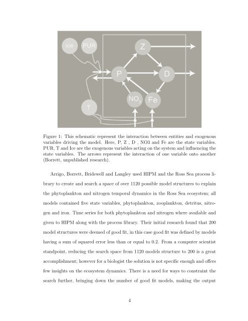
Figure 1: This schematic represent the interaction between entities and exogenous variables driving the model. Here, P, Z , D , NO3 and Fe are the state variables. PUR, T and Ice are the exogenous variables acting on the system and influencing the state variables. The arrows represent the interaction of one variable onto another (Borrett, unpublished research). Arrigo, Borrett, Bridewell and Langley used HIPM and the Ross Sea process library to create and search a space of over 1120 possible model structures to explain the phytoplankton and nitrogen temporal dynamics in the Ross Sea ecosystem; all models contained five state variables, phytoplankton, zooplankton, detritus, nitrogen and iron. Time series for both phytoplankton and nitrogen where available and given to HIPM along with the process library. Their initial research found that 200 model structures were deemed of good fit, in this case good fit was defined by models having a sum of squared error less than or equal to 0.2. From a computer scientist standpoint, reducing the search space from 1120 models structure to 200 is a great accomplishment; however for a biologist the solution is not specific enough and offers few insights on the ecosystem dynamics. There is a need for ways to constraint the search further, bringing down the number of good fit models, making the output 4
Page 1 and 2: HIERARCHAL INDUCTIVE PROCESS MODELI
Page 3 and 4: APPENDIX . . . . . . . . . . . . .
Page 5 and 6: DEDICATION This Thesis is dedicated
Page 7 and 8: LIST OF TABLES 1 Example of entity
Page 9 and 10: LIST OF SYMBOLS P = Amount of Phyto
Page 11: models of natural systems are non-u
Page 15 and 16: specifying the space of possible eq
Page 17 and 18: phytoplankton productivity and comm
Page 19 and 20: 2 METHOD The method employed in thi
Page 21 and 22: set of values that respect the cons
Page 23 and 24: fitted such as for “conc”, with
Page 25 and 26: Table 2: Defining a process - Growt
Page 27 and 28: upon whether certain time-series ar
Page 29 and 30: 3 COMPUTATIONAL RESULTS The main to
Page 31 and 32: ● ● ● 2.0 ● [D,N] ●●●
Page 33 and 34: 3.1 Increase in number of time-seri
Page 35 and 36: Table 4: This table represents each
Page 37 and 38: different restriction powers based
Page 39 and 40: experiment 22, yielding no good fit
Page 41 and 42: not taken into consideration which
Page 43 and 44: Table 5: This table summarizes all
Page 45 and 46: Table 6: This table summarizes all
Page 47 and 48: 4.2 Preliminaries Both Models A and
Page 49 and 50: In addition to these 2 Lemmas, let
Page 51 and 52: When t → ∞ we get the following
Page 53 and 54: For the Zooplankton not to go to ze
Page 55 and 56: ( ∴ P 0 + a ) 13 α − δ Z 0 e
Page 57 and 58: 4.4 Model B Shifting our focus to M
Page 59 and 60: Using the exogenous variables time-
Page 61 and 62: Then finding an lower bound, dD l d
Page 63 and 64:
Thus, using Proposition 1 we get, d
Page 65 and 66:
∴ a 23 = 4.5.10 −4 ≤ F (t)
Page 67 and 68:
Model C Where, dP dt dZ dt dD dt dN
Page 69 and 70:
Next we turn our attention to P (t)
Page 71 and 72:
We can rewrite D u (t) as, D u (t)
Page 73 and 74:
his research on the Ross Sea Phytop
Page 75 and 76:
zooplankton to be properly fitted m
Page 77 and 78:
eally well (Atanasova et al. 2007).
Page 79 and 80:
[9] Dzeroski, S. and Todorovski, L.
Page 81 and 82:
APPENDIX A. Sample CIAO data - 1997
Page 83 and 84:
"death_rate":0.02, "respiration_rat
Page 85 and 86:
"death_rate": (0.02,0.04), "Ek_max"
Page 87 and 88:
# --- GROWTH --- lib.add_generic_pr
Page 89 and 90:
"arrigoetal1998", "light_lim", [("P
Page 91 and 92:
lib.add_generic_process( "death_exp
Page 93 and 94:
lib.add_generic_process( "holling_t
Page 95 and 96:
[], {"max_mixing_rate":(0.000001,1)
Page 97 and 98:
Model E [ dP [ ] dt = (1 − E ice
Page 99 and 100:
Model G [ dP [ ] ( dt = (1 − E ic
Page 101:
BIOGRAPHICAL SKETCH I was born and
show all

HIERARCHAL INDUCTIVE PROCESS MODELING AND ANALYSIS ...

You also want an ePaper? Increase the reach of your titles

Delete template?

Save as template?