Advanced Queueing Theory
Advanced Queueing Theory
Advanced Queueing Theory

Create successful ePaper yourself
Turn your PDF publications into a flip-book with our unique Google optimized e-Paper software.
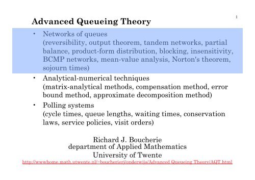
<strong>Advanced</strong> <strong>Queueing</strong> <strong>Theory</strong><br />
1<br />
• Networks of queues<br />
(reversibility, output theorem, tandem networks, partial<br />
balance, product-form distribution, blocking, insensitivity,<br />
BCMP networks, mean-value analysis, Norton's theorem,<br />
sojourn times)<br />
• Analytical-numerical techniques<br />
(matrix-analytical methods, compensation method, error<br />
bound method, approximate decomposition method)<br />
• Polling systems<br />
(cycle times, queue lengths, waiting times, conservation<br />
laws, service policies, visit orders)<br />
Richard J. Boucherie<br />
department of Applied Mathematics<br />
University of Twente<br />
http://wwwhome.math.utwente.nl/~boucherierj/onderwijs/<strong>Advanced</strong> <strong>Queueing</strong> <strong>Theory</strong>/AQT.html
Last time on AQT …<br />
2<br />
• Output reversible queue<br />
• Tandem network of queues<br />
• Jackson network<br />
• Kelly Whittle network<br />
• Partial balance<br />
• Blocking
<strong>Advanced</strong> <strong>Queueing</strong> <strong>Theory</strong><br />
Today (lecture 3): queue length based on Kelly’s<br />
lemma<br />
Nelson, sec 10.4—10.7, Kelly, chapter 3<br />
3<br />
• Kelly Whittle network<br />
• Alternative proof<br />
• Quasi reversibility<br />
• Network of quasi reversible queues<br />
• Queue disciplines, symmetric queues, BCMP networks<br />
• PASTA<br />
• Mean Value Analysis
Kelly Whittle network<br />
4<br />
Theorem: The equilibrium distribution for the Kelly Whittle<br />
network is<br />
where<br />
and π satisfies partial balance
Insert equilibrium distribution and rates in partial balance<br />
5<br />
This is the beauty of partial balance!<br />
rate in = rate out
<strong>Advanced</strong> <strong>Queueing</strong> <strong>Theory</strong><br />
Today (lecture 3): queue length based on Kelly’s<br />
lemma<br />
Nelson, sec 10.4—10.7, Kelly, chapter 3<br />
6<br />
• Kelly Whittle network<br />
• Alternative proof<br />
• Quasi reversibility<br />
• Network of quasi reversible queues<br />
• Queue disciplines, symmetric queues, BCMP networks<br />
• PASTA<br />
• Mean Value Analysis
Time reversed process<br />
7<br />
• Theorem: If X(t) is a stationary Markov process with transition<br />
rates q(j,k), and equilibrium distribution π(j), j ∈ S, then the<br />
reversed process X( τ - t) is a stationary Markov process with<br />
transition rates<br />
and the same equilibrium distribution.<br />
€<br />
• Theorem: Kelly’s lemma<br />
Let X(t) be a stationary Markov process with transition rates<br />
q(j,k). If we can find a collection of numbers q’(j,k) such that<br />
q’(j)=q(j), j ∈S, and a collection of positive numbers π(j),<br />
j ∈ S,<br />
summing to unity, such that<br />
€<br />
€<br />
then q’(j,k) are the transition rates of the time-reversed process,<br />
and (j), j S, is the equilibrium distribution of both processes.<br />
π ∈ € €
Alternative proof: use Kelly’s lemma<br />
8<br />
Forward rates<br />
Guess<br />
backward rates<br />
Check conditions
Alternative proof: use Kelly’s lemma<br />
9<br />
Guess for equilibrium distribution<br />
insert
<strong>Advanced</strong> <strong>Queueing</strong> <strong>Theory</strong><br />
Today (lecture 3): queue length based on Kelly’s<br />
lemma<br />
Nelson, sec 10.4—10.7, Kelly, chapter 3<br />
10<br />
• Kelly Whittle network<br />
• Alternative proof<br />
• Quasi reversibility<br />
• Network of quasi reversible queues<br />
• Queue disciplines, symmetric queues, BCMP networks<br />
• PASTA<br />
• Mean Value Analysis
Quasi-reversibility<br />
• Multi class queueing network, class c<br />
• A queue is quasi-reversible if its state x(t) is a stationary<br />
Markov process with the property that the state of the queue<br />
at time t 0 , x(t 0 ), is independent € of<br />
(i) arrival times of class c customers subsequent to time t 0<br />
(ii) departure times of class c customers prior to time t 0 .<br />
∈<br />
C<br />
• Theorem<br />
If a queue is QR then<br />
(i) arrival times of class c customers form independent<br />
Poisson processes<br />
(ii) departure times of class c customers form independent<br />
Poisson processes.
Quasi-reversibility<br />
• S(c,x) set of states queue contains one more class c<br />
customer than in state x<br />
• Arrival rate class c customer<br />
independent of state x<br />
• Thus arrival rate independent of prior events, and has<br />
constant rate Poisson proces
Quasi-reversibility<br />
• Multi class queueing network, class c<br />
• S(c,x) set of states in which queue contains one more<br />
class c than in state x<br />
• Arrival rate class c customer<br />
independent of state x<br />
€<br />
• Departure rate class c customer<br />
independent of state x<br />
∈<br />
C<br />
• Characterise QR, combine<br />
• Partial balance
<strong>Advanced</strong> <strong>Queueing</strong> <strong>Theory</strong><br />
Today (lecture 3): queue length based on Kelly’s<br />
lemma<br />
Nelson, sec 10.4—10.7, Kelly, chapter 3<br />
14<br />
• Kelly Whittle network<br />
• Alternative proof<br />
• Quasi reversibility<br />
• Network of quasi reversible queues<br />
• Queue disciplines, symmetric queues, BCMP networks<br />
• PASTA<br />
• Mean Value Analysis
Network of quasi reversible queues<br />
• Multiclass queueing network, type i=1,..,I<br />
• J queues<br />
• Customer type identifies route<br />
• Poisson arrival rate per type (i), i=1,…,I<br />
• Route r(i,1),r(i,2),…,r(i,S(i))<br />
• Type i at stage s in queue r(i,s)<br />
• S(c,x) set of states in which queue contains one more class c<br />
than in state x<br />
15<br />
• State X(t)=(x 1 (t),…,x J (t))<br />
• Fixed number of visits; cannot use Markov routing<br />
• 1, 2, or 3 visits to queue: use 3 types
Network of quasi reversible queues<br />
16<br />
• Construct network by multiplying rates for individual queues<br />
• Transition rates<br />
• Arrival of type i causes queue k=r(i,1) to change at<br />
• Departure type i from queue j = r(i,S(i))<br />
• Routing<br />
• Internal
• Rates<br />
Network of Quasi-reversible queues<br />
• Theorem : For an open network of QR queues<br />
(i) the states of individual queues are independent at fixed time<br />
(ii) an arriving customer sees the equilibrium distribution<br />
(ii’) the equibrium distribution for a queue is as it would be in<br />
isolation with arrivals forming a Poisson process.<br />
(iii) time-reversal: another open network of QR queues<br />
(iv) system is QR, so departures form Poisson process
Network of Quasi-reversible queues<br />
• Proof of part (i): Kelly’s lemma<br />
• Rates<br />
• Transition rates reversed process (guess)
Network of Quasi-reversible queues<br />
• Proof of part (i): Kelly’s lemma<br />
• For<br />
• We have<br />
• Satisfied due to
<strong>Advanced</strong> <strong>Queueing</strong> <strong>Theory</strong><br />
Today (lecture 3): queue length based on Kelly’s<br />
lemma<br />
Nelson, sec 10.4—10.7, Kelly, chapter 3<br />
20<br />
• Kelly Whittle network<br />
• Alternative proof<br />
• Quasi reversibility<br />
• Network of quasi reversible queues<br />
• Queue disciplines, symmetric queues, BCMP networks<br />
• PASTA<br />
• Mean Value Analysis
Queue disciplines<br />
• Operation of the queue j:<br />
(i) Each job requires exponential(1) amount of service.<br />
(ii) Total service effort supplied at rate ϕ j (n j )<br />
(iii) Proportion γ j (k,n j ) of this effort directed to job in<br />
position k, k=1,…, n j ; when this job leaves, his service is<br />
completed, jobs in positions k+1,…, n j move to positions k,…,<br />
n j -1.<br />
(iv) When a job arrives at queue j he moves into position k<br />
with probability j (k,n j + 1),<br />
k=1,…, n j +1; jobs previously in positions k,…, n j move to<br />
positions k+1,…, n j +1.
Queue disciplines<br />
• Operation of the queue j:<br />
(i) Each job requires exponential(1) amount of service.<br />
(ii) Total service effort supplied at rate ϕ j (n j )<br />
(iii) Proportion j (k,n j ) of this effort directed to job in position<br />
k,<br />
(iv) job arriving at queue j moves into position k with prob.<br />
j (k,n j + 1)<br />
• In the form of network of quasi reversible queues<br />
• Examples: BCMP network<br />
FCFS<br />
LCFS<br />
PS<br />
infinite server queue,
Symmetric queues<br />
• Operation of the queue j:<br />
(i) Each job requires exponential(1) amount of service.<br />
(ii) Total service effort supplied at rate ϕ j (n j )<br />
(iii) Proportion j (k,n j ) of this effort directed to job in position<br />
k,<br />
(iv) job arriving at queue j moves into position k with prob.<br />
j (k,n j + 1)<br />
• Examples: IS, LCFS, PS<br />
• Symmetric queue QR for general service requirement<br />
• Instantaneous attention<br />
• Symmetric queue is insensitive
Quasi-reversibility and partial balance<br />
• QR: fairly general queues, service disciplines, Markov<br />
routing, product form equilibrium distribution<br />
factorizes over queues.<br />
• PB: fairly general relation between service rate at<br />
queues, state-dependent routing (blocking), product<br />
form equilibrium distribution factorizes over service<br />
and routing parts.<br />
• Identical for single type queueing network with<br />
Markov routing<br />
• QR partial balance<br />
• NOT partial balance QR (exercise)<br />
• NOT QR Reversibility (see Nelson, ex 10.14)<br />
• NOT Reversibility QR (see Nelson, ex 10.12)
<strong>Advanced</strong> <strong>Queueing</strong> <strong>Theory</strong><br />
Today (lecture 3): queue length based on Kelly’s<br />
lemma<br />
Nelson, sec 10.4—10.7, Kelly, chapter 3<br />
25<br />
• Kelly Whittle network<br />
• Alternative proof<br />
• Quasi reversibility<br />
• Network of quasi reversible queues<br />
• Queue disciplines, symmetric queues, BCMP networks<br />
• PASTA<br />
• Mean Value Analysis
Arrival theorem<br />
• PASTA:<br />
The distribution of the number of customers in the system seen by a<br />
a customer arriving to a system according to a Poisson process (i.e.,<br />
at an arrival epoch) equals the distribution of the number of<br />
customers at an arbitrary epoch.<br />
• Arrival theorem (open Jackson network):<br />
In an open network in equilibrium, a customer arriving to queue j<br />
observes the equilibrium distribution.<br />
• Arrival theorem (closed Jackson network):<br />
In a closed networkin equilibrium, a customer arriving to queue j<br />
observes the equilibrium distribution of the network containing one<br />
customer less.
PASTA: Poisson Arrivals See Time Averages <br />
27<br />
• fraction of time system in state n<br />
• probability outside observer sees n customers at time t<br />
• probability that arriving customer sees n customers at time t<br />
(just before arrival at time t there are n customers in the system)<br />
• in general
28<br />
PASTA: Poisson Arrivals See Time Averages <br />
• Let C(t,t+h) event customer arrives in (t,t+h)<br />
• For Poisson arrivals q(n,n+1)= so that<br />
• Alternative explanation; PASTA holds in general!
29<br />
PASTA: Poisson Arrivals See Time Averages <br />
• Transient<br />
• In equilibrium
30<br />
MUSTA: Moving Units See Time Averages <br />
• Palm probabilities: <br />
Each type of transition nnʼ for Markov chain associated with subset H of SxS \diag(SxS)<br />
• Example:transition in which customer queue i queue j<br />
H ij<br />
=<br />
• Transition in which customer leaves queue i<br />
H<br />
i<br />
out<br />
{(m + e i<br />
,m + e j<br />
),m + e i<br />
,m + e j<br />
∈ S}<br />
m<br />
=<br />
H ij<br />
j<br />
• Transition in which customer enters queue j<br />
H in j<br />
=<br />
H ij<br />
i
31<br />
MUSTA: Moving Units See Time Averages <br />
• N H process counting the H-transitions <br />
• Palm probability P H (C) of event C given that H occurs: <br />
P H<br />
(C) =<br />
∑(n,n')∈C<br />
π(n)q(n,n')<br />
∑ π(n)q(n,n') , C ⊆ H<br />
(n,n')∈ H<br />
• Probability customer queue i queue j sees state m<br />
P ij<br />
(m) = P H ij<br />
((m + e i<br />
,m + e j<br />
)) = π(m + e )q(m + e ,m + e )<br />
i i j<br />
,<br />
π(n)q(n,n')<br />
∑(n,n')∈ H ij<br />
• Probability customer arriving to queue j sees state m<br />
P j<br />
(m) = P H j<br />
in (<br />
(m + e i<br />
,m + e j<br />
)) =<br />
i<br />
∑ π(m + e<br />
i<br />
i<br />
)q(m + e i<br />
,m + e j<br />
)<br />
∑<br />
i<br />
∑ π(n)q(n,n') ,<br />
(n,n')∈ H ij
Kelly Whittle network<br />
32<br />
Theorem: The equilibrium distribution for the Kelly Whittle<br />
network is<br />
where<br />
and π satisfies partial balance
MUSTA :Kelly Whittle network<br />
33<br />
Theorem: The distribution seen by a customer<br />
moving from queue i tot queue j is<br />
Entering queue j is<br />
where
MUSTA <br />
34
<strong>Advanced</strong> <strong>Queueing</strong> <strong>Theory</strong><br />
Today (lecture 3): queue length based on Kelly’s<br />
lemma<br />
Nelson, sec 10.4—10.7, Kelly, chapter 3<br />
35<br />
• Kelly Whittle network<br />
• Alternative proof<br />
• Quasi reversibility<br />
• Network of quasi reversible queues<br />
• Queue disciplines, symmetric queues, BCMP networks<br />
• PASTA<br />
• Mean Value Analysis
Gesloten netwerken: MVA<br />
Average queue length, average sojourn times<br />
λ m (i) arrival intensity queue i,<br />
F m (i) expeceted sojourn time i,<br />
L m (i) expected queue length queue i, when m cust in system<br />
Arrival theorem, FCFS<br />
Little’s formula
Gesloten netwerken: MVA<br />
λ m (i) arrival intensity queue i,<br />
F m (i) expeceted sojourn time i,<br />
L m (i) expected queue length queue i, when m cust in system<br />
€<br />
€<br />
• Little<br />
• thus<br />
λ m<br />
(i) =<br />
N<br />
∑<br />
j=1<br />
λ m<br />
( j) ⋅ r ji<br />
€<br />
π i<br />
=<br />
λ m<br />
(i) = λ m<br />
⋅ π i<br />
, λ m<br />
= λ m<br />
(i)<br />
N<br />
∑<br />
i=1<br />
⎧<br />
λ m<br />
= m ⋅ ⎨<br />
⎩<br />
N<br />
∑<br />
i=1<br />
N<br />
∑ π j<br />
⋅ r ji<br />
, ∑ π i<br />
=1<br />
j=1<br />
⎫<br />
π i<br />
⋅ F m<br />
(i) ⎬<br />
⎭<br />
−1<br />
N<br />
i=1
• Mean Value Analysis<br />
evaluates λ m (i), F m (i) en L m (i) for all m,i recursively<br />
– Find solution π of traffic equations<br />
– for m=1 : F 1 (i)=1/µ i for all i<br />
recursion<br />
– let F m (i) known for all i<br />
– Determine number of cust served per time unit at queue i :<br />
λ m<br />
(i) = λ m<br />
⋅ π i<br />
= m ⋅<br />
{ ∑<br />
N<br />
π<br />
j=1 j<br />
⋅ F m<br />
( j) } −1 ⋅ π i<br />
– Determine average number of customers at queue i<br />
using Little<br />
– Determine average sojourn time at queue i for system<br />
€ containing m+1 customers using arrival theorem<br />
F m +1<br />
(i) = 1+ L m(i)<br />
µ i<br />
€<br />
L m<br />
(i) = λ m<br />
(i) ⋅ F m<br />
(i)
Exercises<br />
Exercises from Kelly, Reversibility and stochastic networks: 1.5.2, 1.6.4, 2.2.4, 2.3.5, 2.4.1, 3.1.3, 3.1.4, 3.2.3<br />
Exercise on blocking: Consider a Jackson network of J queues with transition rates<br />
1. Give the equilibrium distribution, and show that this distribution satisfies partial balance<br />
2. Show that a customer arriving to queue i observes the equilibrium distribution<br />
3. Now assume that the total number of customer in the network is restricted not to exceed N. Give the<br />
equilibrium distribution, and the distribution of the state observed by a customer arriving to queue 1<br />
4. Now assume that each queue has a capacity restriction, say the number in queue i is restricted not to exceed Ni.<br />
Consider the stop protocol, where the arrival process, and each non-blocked queue is stopped until a service<br />
completion has occurred at the blocked queue. Give the state space, and show that the equilibrium distribution<br />
has a product form and satisfies partial balance. Give the distribution of the state observed by a customer<br />
arriving to (and entering) queue 1.<br />
5. Again assume the capacity restrictions of 4). Assume that a customer arriving to a queue that has reached its<br />
capacity restriction, say queue j, jumps over the queue, and selects a new destination according to the routing<br />
probilities from queue j. Give the equilibrium distribution.<br />
6. Can the product form result of 4) be obtained via Quasi reversibility If so, provide the proof of the product form<br />
result via quasi reversibility.<br />
Exercise on insensitivity: Consider a BCMP network consisting of infinite server queues, and single server queues,<br />
where the single server queues may be FCFS, LCFS or PS. Assume Markov routing.<br />
1. Formule the BCMP network as a network of quasi reversible queues.<br />
2. Give the equilibrium distribution.<br />
3. Show that this distribution satisfies partial balance.<br />
4. Restrict the network to contain IS, LCFS, and PS queues only (symmetric queues). Prove that the equilibrium<br />
is insensitive to the distibution of the service time at each of these queues using first the phase type<br />
distribution approach, and then the formulation of Whittle.<br />
5. Indicate why the distribution cannot be insensitive to the service time distribution in an FCFS queue.