Minimal Models of Adapted Neuronal Response to In Vivo–Like ...
Minimal Models of Adapted Neuronal Response to In Vivo–Like ...
Minimal Models of Adapted Neuronal Response to In Vivo–Like ...

You also want an ePaper? Increase the reach of your titles
YUMPU automatically turns print PDFs into web optimized ePapers that Google loves.
2112 G. La Camera, A. Rauch, H.-R. Lüscher, W. Senn, and S. Fusi<br />
firing rate [Hz]<br />
30<br />
20<br />
10<br />
0<br />
30<br />
20<br />
10<br />
0<br />
CELL A CELL B<br />
20<br />
10<br />
0<br />
20<br />
10<br />
0 200 400<br />
0<br />
0 200 400<br />
m [pA]<br />
AHP<br />
AT<br />
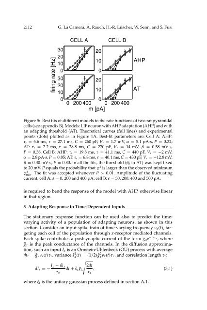
Figure 5: Best fits <strong>of</strong> different models <strong>to</strong> the rate functions <strong>of</strong> two rat pyramidal<br />
cells (see appendix B). <strong>Models</strong>: LIF neuron with AHP adaptation (AHP) and with<br />
an adapting threshold (AT). Theoretical curves (full lines) and experimental<br />
points (dots) plotted as in Figure 1A. Best-fit parameters are: Cell A: AHP:<br />
τ r = 6.6 ms, τ = 27.1 ms, C = 260 pF, V r = 1.7 mV,α = 5.1 pA·s, P = 0.32;<br />
AT: τ r = 2.2 ms, τ = 28.8 ms, C = 270 pF, V r = 14 mV, β = 0.58 mV·s,<br />
P = 0.38. Cell B: AHP: τ r = 19.8 ms, τ = 41.1 ms, C = 440 pF, V r =−2mV,<br />
α = 2.8pA·s, P = 0.85; AT: τ r = 6.8 ms, τ = 40.1 ms, C = 430 pF, V r =−12.8mV,<br />
β = 0.30 mV·s, P = 0.80. <strong>In</strong> all the fits, the threshold (θ 0 in AT) was kept fixed<br />
<strong>to</strong> 20 mV. P equals the probability that χ 2 is larger than the observed minimum<br />
χmin 2 . The fit was accepted whenever P > 0.01. Amplitude <strong>of</strong> the fluctuating<br />
current: cell A: s = 0, 200 and 400 pA; cell B: s = 50, 200, 400 and 500 pA.<br />
is required <strong>to</strong> bend the response <strong>of</strong> the model with AHP, otherwise linear<br />
in that region.<br />
3 Adapting <strong>Response</strong> <strong>to</strong> Time-Dependent <strong>In</strong>puts<br />
The stationary response function can be used also <strong>to</strong> predict the timevarying<br />
activity <strong>of</strong> a population <strong>of</strong> adapting neurons, as shown in this<br />
section. Consider an input spike train <strong>of</strong> time-varying frequency ν x (t), targeting<br />
each cell <strong>of</strong> the population through x-recep<strong>to</strong>r mediated channels.<br />
Each spike contributes a postsynaptic current <strong>of</strong> the form ḡ x e −t/τ x<br />
, where<br />
ḡ x is the peak conductance <strong>of</strong> the channels. <strong>In</strong> the diffusion approximation,<br />
such an input I x is an Ornstein-Uhlenbeck (OU) process with average<br />
¯m x = ḡ x ν x (t)τ x , variance ¯s 2 x (t) = (1/2)ḡ2 x ν x(t)τ x , and correlation length τ x :<br />
√<br />
dI x =− I x − ¯m x 2dt<br />
dt + ¯s x ξ t , (3.1)<br />
τ x<br />
τ x<br />
where ξ t is the unitary gaussian process defined in section A.1.