Minimal Models of Adapted Neuronal Response to In Vivo–Like ...

More documents

Recommendations

Info

2108 G. La Camera, A. Rauch, H.-R. Lüscher, W. Senn, and S. Fusi fixed point of the self-consistent equation, where f = CB (m 0 − αf, s 0 ), (2.5) ⎡ ⎤ ∫ Cθ−m 0 τ∗ CB = ⎣τ r + τ ∗ √ s 0 τ ∗ √ πe x 2 (1 + erf(x))dx⎦ CVr−m 0 τ ∗ s 0 √ τ ∗ −1 . (2.6) CB is the rate function of the CB neuron (Burkitt, Meffin, & Grayden, 2003). Note that the only difference with the response function of the current-based LIF neuron, equation 2.3, is in the dependence of the quantities m 0 , s 0 ,τ ∗ , given, respectively, by equations A.10, A.11, and A.6, upon the input parameters ḡ E,I , ν E,I . Here ḡ E,I are the excitatory and inhibitatory peak conductances and ν E,I the mean frequencies of the input spike trains, modeled as Poisson processes. Equations A.10 and A.11 have to be compared with m = ḡ E ν E − ḡ I ν I , s 2 = ḡ 2 E ν E + ḡ 2 I ν I, valid for the current-based neuron. Note that one way to obtain the plots of Figure 1A is to increase ν E while scaling ḡ E as A/ √ ν E , with A held constant and for constant inhibition (i.e., for constant ḡ I , ν I ). This in fact corresponds to increasing m as A √ ν E − ḡ I ν I at constant noise s 2 = A 2 + ḡ 2 I ν I. To make a comparison with the current-based neuron, we plotted CB as a function of µ E = ḡ E ν E according to such a procedure in Figure 3, which presents the match between the predictions of the rate model and simulations of the adapting CB neuron. 2.1.4 Other Model Neurons. A similar agreement is obtained for other IF model neurons (results not shown). Particularly worth mentioning is the constant leakage IF neuron with a floor (CLIFF) (Fusi & Mattia, 1999; Rauch et al., 2003), whose response function is very simple and does not require any integration: [ σ 2 ( ) (m, s) = τ r + 2(m − λ) 2 e − 2Cθ(m−λ) σ 2 − e − 2CVr(m−λ) σ 2 + C(θ − V ] −1 r) . m − λ The input parameters m, σ are defined as for the LIF neuron. The CLIFF neuron is an LIF neuron with constant leakage (i.e., with the term −(V − V rest )/τ in equation A.1 replaced by the constant −λ/C), and a reflecting barrier for the the membrane potential (Fusi & Mattia, 1999). However, the scheme proposed here to derive the adapting rate models does not apply to IF neurons only. For example, the response function of a Hodgkin-Huxley neuron with an A-current can be fitted by the simple model 1 = a[m − m th ] + − b[m − m th ] 2 + (Shriki et al., 2003), where a, b
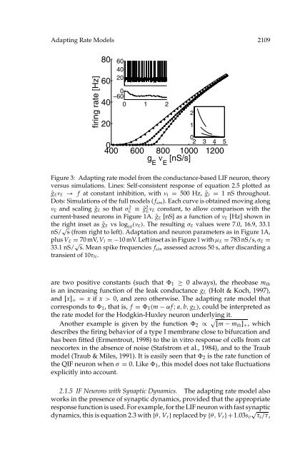
Adapting Rate Models 2109 firing rate [Hz] 80 60 40 20 60 40 20 −60 0 0 1 2 0 2 3 4 5 0 400 600 800 1000 1200 g E ν E [nS/s] 2 1 Figure 3: Adapting rate model from the conductance-based LIF neuron, theory versus simulations. Lines: Self-consistent response of equation 2.5 plotted as ḡ E ν E → f at constant inhibition, with ν I = 500 Hz, ḡ I = 1 nS throughout. Dots: Simulations of the full models ( f sim ). Each curve is obtained moving along ν E and scaling ḡ E so that σE 2 ≡ ḡ2 E ν E constant, to allow comparison with the current-based neurons in Figure 1A. ḡ E [nS] as a function of ν E [Hz] shown in the right inset as ḡ E vs log 10 (ν E ). The resulting σ E values were 7.0, 16.9, 33.1 nS/ √ s (from right to left). Adaptation and neuron parameters as in Figure 1A, plus V E = 70 mV, V I =−10 mV. Left inset as in Figure 1 with µ E = 783 nS/s, σ E = 33.1 nS/ √ s. Mean spike frequencies f sim assessed across 50 s, after discarding a transient of 10τ N . are two positive constants (such that 1 ≥ 0 always), the rheobase m th is an increasing function of the leak conductance g L (Holt & Koch, 1997), and [x] + = x if x > 0, and zero otherwise. The adapting rate model that corresponds to 1 , that is, f = 1 (m − αf ; a, b, g L ), could be interpreted as the rate model for the Hodgkin-Huxley neuron underlying it. Another example is given by the function 2 ∝ √ [m − m th ] + , which describes the firing behavior of a type I membrane close to bifurcation and has been fitted (Ermentrout, 1998) to the in vitro response of cells from cat neocortex in the absence of noise (Stafstrom et al., 1984), and to the Traub model (Traub & Miles, 1991). It is easily seen that 2 is the rate function of the QIF neuron when σ = 0. Like 1 , this model does not take fluctuations explicitly into account. 2.1.5 IF Neurons with Synaptic Dynamics. The adapting rate model also works in the presence of synaptic dynamics, provided that the appropriate response function is used. For example, for the LIF neuron with fast synaptic dynamics, this is equation 2.3 with {θ,V r } replaced by {θ,V r }+1.03s v √ τs /τ,
Page 1 and 2: LETTER Communicated by Bard Ermentr
Page 3 and 4: Adapting Rate Models 2103 We show t
Page 5 and 6: Adapting Rate Models 2105 the self-
Page 7: Adapting Rate Models 2107 firing ra
Page 11 and 12: Adapting Rate Models 2111 firing ra
Page 13 and 14: Adapting Rate Models 2113 Table 1:
Page 15 and 16: Adapting Rate Models 2115 The maxim
Page 17 and 18: Adapting Rate Models 2117 I ahp =
Page 19 and 20: Adapting Rate Models 2119 with µ s
Page 21 and 22: Adapting Rate Models 2121 Reference
Page 23 and 24: Adapting Rate Models 2123 Powers, R

Minimal Models of Adapted Neuronal Response to In Vivo–Like ...

You also want an ePaper? Increase the reach of your titles

Delete template?

Save as template?