Minimal Models of Adapted Neuronal Response to In Vivo–Like ...

2108 G. La Camera, A. Rauch, H.-R. Lüscher, W. Senn, and S. Fusi
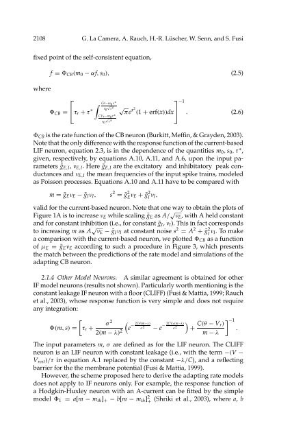
fixed point of the self-consistent equation,
where
f = CB (m 0 − αf, s 0 ), (2.5)
⎡
⎤
∫ Cθ−m 0 τ∗
CB = ⎣τ r + τ ∗ √
s 0 τ ∗ √ πe
x 2 (1 + erf(x))dx⎦
CVr−m 0 τ ∗
s 0
√
τ ∗
−1
. (2.6)
CB is the rate function of the CB neuron (Burkitt, Meffin, & Grayden, 2003).
Note that the only difference with the response function of the current-based
LIF neuron, equation 2.3, is in the dependence of the quantities m 0 , s 0 ,τ ∗ ,
given, respectively, by equations A.10, A.11, and A.6, upon the input parameters
ḡ E,I , ν E,I . Here ḡ E,I are the excitatory and inhibitatory peak conductances
and ν E,I the mean frequencies of the input spike trains, modeled
as Poisson processes. Equations A.10 and A.11 have to be compared with
m = ḡ E ν E − ḡ I ν I , s 2 = ḡ 2 E ν E + ḡ 2 I ν I,
valid for the current-based neuron. Note that one way to obtain the plots of
Figure 1A is to increase ν E while scaling ḡ E as A/ √ ν E , with A held constant
and for constant inhibition (i.e., for constant ḡ I , ν I ). This in fact corresponds
to increasing m as A √ ν E − ḡ I ν I at constant noise s 2 = A 2 + ḡ 2 I ν I. To make
a comparison with the current-based neuron, we plotted CB as a function
of µ E = ḡ E ν E according to such a procedure in Figure 3, which presents
the match between the predictions of the rate model and simulations of the
adapting CB neuron.
2.1.4 Other Model Neurons. A similar agreement is obtained for other
IF model neurons (results not shown). Particularly worth mentioning is the
constant leakage IF neuron with a floor (CLIFF) (Fusi & Mattia, 1999; Rauch
et al., 2003), whose response function is very simple and does not require
any integration:
[
σ 2 (
)
(m, s) = τ r +
2(m − λ) 2 e − 2Cθ(m−λ)
σ 2 − e − 2CVr(m−λ)
σ 2 + C(θ − V ] −1
r)
.
m − λ
The input parameters m, σ are defined as for the LIF neuron. The CLIFF
neuron is an LIF neuron with constant leakage (i.e., with the term −(V −
V rest )/τ in equation A.1 replaced by the constant −λ/C), and a reflecting
barrier for the the membrane potential (Fusi & Mattia, 1999).
However, the scheme proposed here to derive the adapting rate models
does not apply to IF neurons only. For example, the response function of
a Hodgkin-Huxley neuron with an A-current can be fitted by the simple
model 1 = a[m − m th ] + − b[m − m th ] 2 + (Shriki et al., 2003), where a, b