"WINNER II Channel Models", ver 1.1, Sept

WINNER II D1.1.2 V1.1
( τ ' − min( τ '))
τ = sort
. (4.2)
n
n
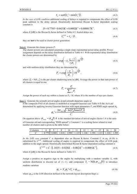
In the case of LOS condition additional scaling of delays is required to compensate the effect of LOS
peak addition to the delay spread. Heuristically determined Ricean K-factor dependent scaling
constant is
D +
n
2
3
= 0.7705−
0.0433K
+ 0.0002K
0.000017K
, (4.3)
where K [dB] is the Ricean K-factor defined in Table 4-5. Scaled delays are
LOS
τ = τ D , (4.4)
n n
/
they are not to be used in cluster power generation.
Step 6: Generate the cluster powers P.
The cluster powers are calculated assuming a single slope exponential power delay profile. Power
assignment depends on the delay distribution defined in Table 4-5. With exponential delay distribution
the cluster powers are determined by
'
⎛
Pn
= exp
⎜−
⎝
n
r 1⎞
τ
−
10
r
⎟ ⋅
τστ
⎠
and with uniform delay distribution they are determined by
'
P n
−Ζ
10
n
τ (4.5)
⎛ −τ
⎞
n
= exp
⎜
⎟ ⋅ 10
⎝ σ τ ⎠
−Ζ
10
n
, (4.6)
where Ζ n ~ N(0, ζ ) is the per cluster shadowing term in [dB]. Average the power so that sum power of
all clusters is equal to one
P
'
n
n
=
N
∑ n = 1
P
Assign the power of each ray within a cluster as P n / M, where M is the number of rays per cluster.
Step 7: Generate the azimuth arrival angles ϕ and azimuth departure angles φ.
If the composite PAS of all clusters is modelled as wrapped Gaussian (see Table 4-5) the AoA are
determined by applying inverse Gaussian function with input parameters P n and RMS angle spread σ ϕ
On equation above 1. 4
AoA
2 ln
' = σ AoA
−
C
P
'
n
( P max( P ))
(4.7)
n
n
ϕ
n
. (4.8)
σ = σ is the standard deviation of arrival angles (factor 1.4 is the ratio
ϕ
of Gaussian std and corresponding ”RMS spread”). Constant C is a scaling factor related to total
number of clusters and is given in the table below:
# clusters 4 5 8 10 11 12 14 15 16 20
C 0.779 0.860 1.018 1.090 1.123 1.146 1.190 1.211 1.226 1.289
In the LOS case constant C is dependent also on Ricean K-factor. Constant C in eq. (4.10) is
substituted by C LOS . Additional scaling of angles is required to compensate the effect of LOS peak
addition to the angle spread. Heuristically determined Ricean K-factor dependent scaling constant is
2
3
( 1.1035
− 0.028K
− 0.002K
0.0001K
)
C LOS C ⋅
+
= , (4.9)
where K [dB] is the Ricean K-factor defined in Table 4-5.
Assign a positive or negative sign to the angles by multiplying with a random variable X n with
uniform distribution to discrete set of {1,–1}, add component N( 0, 5)
random variation
n
n
n
n
LOS
n
~
AoA
Y σ to introduce
ϕ = X ϕ ' + Y + ϕ , (4.10)
where ϕ LOS is the LOS direction defined in the network layout description Step1.c.
Page 39 (82)