The caret Package - NexTag Supports Open Source Initiatives
The caret Package - NexTag Supports Open Source Initiatives
The caret Package - NexTag Supports Open Source Initiatives
You also want an ePaper? Increase the reach of your titles
YUMPU automatically turns print PDFs into web optimized ePapers that Google loves.
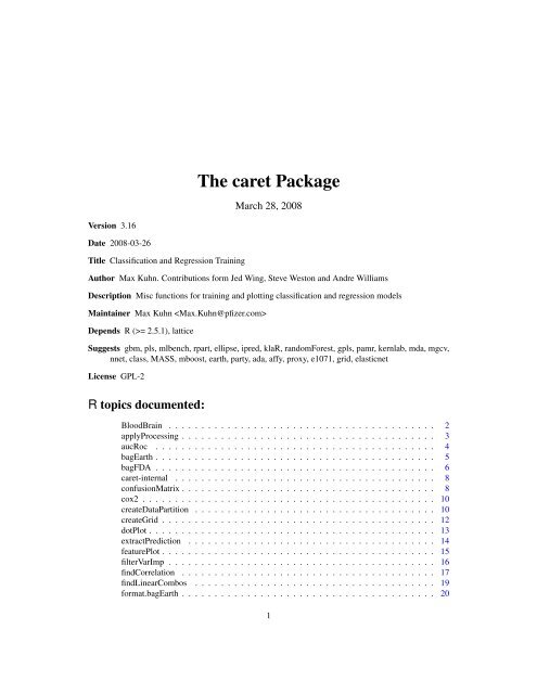
<strong>The</strong> <strong>caret</strong> <strong>Package</strong><br />
March 28, 2008<br />
Version 3.16<br />
Date 2008-03-26<br />
Title Classification and Regression Training<br />
Author Max Kuhn. Contributions form Jed Wing, Steve Weston and Andre Williams<br />
Description Misc functions for training and plotting classification and regression models<br />
Maintainer Max Kuhn <br />
Depends R (>= 2.5.1), lattice<br />
Suggests gbm, pls, mlbench, rpart, ellipse, ipred, klaR, randomForest, gpls, pamr, kernlab, mda, mgcv,<br />
nnet, class, MASS, mboost, earth, party, ada, affy, proxy, e1071, grid, elasticnet<br />
License GPL-2<br />
R topics documented:<br />
BloodBrain . . . . . . . . . . . . . . . . . . . . . . . . . . . . . . . . . . . . . . . . . 2<br />
applyProcessing . . . . . . . . . . . . . . . . . . . . . . . . . . . . . . . . . . . . . . . 3<br />
aucRoc . . . . . . . . . . . . . . . . . . . . . . . . . . . . . . . . . . . . . . . . . . . 4<br />
bagEarth . . . . . . . . . . . . . . . . . . . . . . . . . . . . . . . . . . . . . . . . . . . 5<br />
bagFDA . . . . . . . . . . . . . . . . . . . . . . . . . . . . . . . . . . . . . . . . . . . 6<br />
<strong>caret</strong>-internal . . . . . . . . . . . . . . . . . . . . . . . . . . . . . . . . . . . . . . . . 8<br />
confusionMatrix . . . . . . . . . . . . . . . . . . . . . . . . . . . . . . . . . . . . . . . 8<br />
cox2 . . . . . . . . . . . . . . . . . . . . . . . . . . . . . . . . . . . . . . . . . . . . . 10<br />
createDataPartition . . . . . . . . . . . . . . . . . . . . . . . . . . . . . . . . . . . . . 10<br />
createGrid . . . . . . . . . . . . . . . . . . . . . . . . . . . . . . . . . . . . . . . . . . 12<br />
dotPlot . . . . . . . . . . . . . . . . . . . . . . . . . . . . . . . . . . . . . . . . . . . . 13<br />
extractPrediction . . . . . . . . . . . . . . . . . . . . . . . . . . . . . . . . . . . . . . 14<br />
featurePlot . . . . . . . . . . . . . . . . . . . . . . . . . . . . . . . . . . . . . . . . . . 15<br />
filterVarImp . . . . . . . . . . . . . . . . . . . . . . . . . . . . . . . . . . . . . . . . . 16<br />
findCorrelation . . . . . . . . . . . . . . . . . . . . . . . . . . . . . . . . . . . . . . . 17<br />
findLinearCombos . . . . . . . . . . . . . . . . . . . . . . . . . . . . . . . . . . . . . 19<br />
format.bagEarth . . . . . . . . . . . . . . . . . . . . . . . . . . . . . . . . . . . . . . . 20<br />
1
2 BloodBrain<br />
Alternate Affy Gene Expression Summary Methods. . . . . . . . . . . . . . . . . . . . 21<br />
knn3 . . . . . . . . . . . . . . . . . . . . . . . . . . . . . . . . . . . . . . . . . . . . . 22<br />
maxDissim . . . . . . . . . . . . . . . . . . . . . . . . . . . . . . . . . . . . . . . . . 24<br />
mdrr . . . . . . . . . . . . . . . . . . . . . . . . . . . . . . . . . . . . . . . . . . . . . 26<br />
nearZeroVar . . . . . . . . . . . . . . . . . . . . . . . . . . . . . . . . . . . . . . . . . 27<br />
normalize.AffyBatch.normalize2Reference . . . . . . . . . . . . . . . . . . . . . . . . 28<br />
normalize2Reference . . . . . . . . . . . . . . . . . . . . . . . . . . . . . . . . . . . . 29<br />
oil . . . . . . . . . . . . . . . . . . . . . . . . . . . . . . . . . . . . . . . . . . . . . . 31<br />
panel.needle . . . . . . . . . . . . . . . . . . . . . . . . . . . . . . . . . . . . . . . . . 31<br />
plot.train . . . . . . . . . . . . . . . . . . . . . . . . . . . . . . . . . . . . . . . . . . . 32<br />
plot.varImp.train . . . . . . . . . . . . . . . . . . . . . . . . . . . . . . . . . . . . . . 34<br />
plotClassProbs . . . . . . . . . . . . . . . . . . . . . . . . . . . . . . . . . . . . . . . 35<br />
plotObsVsPred . . . . . . . . . . . . . . . . . . . . . . . . . . . . . . . . . . . . . . . 36<br />
plsda . . . . . . . . . . . . . . . . . . . . . . . . . . . . . . . . . . . . . . . . . . . . . 37<br />
postResample . . . . . . . . . . . . . . . . . . . . . . . . . . . . . . . . . . . . . . . . 39<br />
pottery . . . . . . . . . . . . . . . . . . . . . . . . . . . . . . . . . . . . . . . . . . . . 40<br />
preProcess . . . . . . . . . . . . . . . . . . . . . . . . . . . . . . . . . . . . . . . . . . 40<br />
predict.bagEarth . . . . . . . . . . . . . . . . . . . . . . . . . . . . . . . . . . . . . . . 42<br />
predict.knn3 . . . . . . . . . . . . . . . . . . . . . . . . . . . . . . . . . . . . . . . . . 43<br />
print.confusionMatrix . . . . . . . . . . . . . . . . . . . . . . . . . . . . . . . . . . . . 44<br />
print.train . . . . . . . . . . . . . . . . . . . . . . . . . . . . . . . . . . . . . . . . . . 44<br />
resampleHist . . . . . . . . . . . . . . . . . . . . . . . . . . . . . . . . . . . . . . . . 45<br />
resampleSummary . . . . . . . . . . . . . . . . . . . . . . . . . . . . . . . . . . . . . 46<br />
roc . . . . . . . . . . . . . . . . . . . . . . . . . . . . . . . . . . . . . . . . . . . . . . 47<br />
sensitivity . . . . . . . . . . . . . . . . . . . . . . . . . . . . . . . . . . . . . . . . . . 48<br />
spatialSign . . . . . . . . . . . . . . . . . . . . . . . . . . . . . . . . . . . . . . . . . . 50<br />
summary.bagEarth . . . . . . . . . . . . . . . . . . . . . . . . . . . . . . . . . . . . . 51<br />
tecator . . . . . . . . . . . . . . . . . . . . . . . . . . . . . . . . . . . . . . . . . . . . 52<br />
train . . . . . . . . . . . . . . . . . . . . . . . . . . . . . . . . . . . . . . . . . . . . . 53<br />
trainControl . . . . . . . . . . . . . . . . . . . . . . . . . . . . . . . . . . . . . . . . . 56<br />
varImp . . . . . . . . . . . . . . . . . . . . . . . . . . . . . . . . . . . . . . . . . . . . 57<br />
Index 60<br />
BloodBrain<br />
Blood Brain Barrier Data<br />
Description<br />
Mente and Lombardo (2005) develop models to predict the log of the ratio of the concentration<br />
of a compound in the brain and the concentration in blood. For each compound, they computed<br />
three sets of molecular descriptors: MOE 2D, rule-of-five and Charge Polar Surface Area (CPSA).<br />
In all, 134 descriptors were calcualted. Included in this package are 208 non-proprietary literature<br />
compounds. <strong>The</strong> vector logBBB contains the concentration ratio and the data fame bbbDescr<br />
contains the descriptor values.
applyProcessing 3<br />
Usage<br />
Value<br />
data(BloodBrain)<br />
bbbDescr<br />
logBBB<br />
data frame of chemical descriptros<br />
vector of assay results<br />
<strong>Source</strong><br />
Mente, S.R. and Lombardo, F. (2005). A recursive-partitioning model for blood-brain barrier permeation,<br />
Journal of Computer-Aided Molecular Design, Vol. 19, pg. 465–481.<br />
applyProcessing<br />
Data Processing on Predictor Variables (Deprecated)<br />
Description<br />
Usage<br />
processData is used to estimate data processing parameters and applyProcessing takes<br />
the results and applies them to data objects<br />
processData(x, center = TRUE, scale = TRUE, na.remove = TRUE)<br />
applyProcessing(x, object)<br />
Arguments<br />
x<br />
center<br />
scale<br />
na.remove<br />
object<br />
A matrix or data frame with variables in rows and samples in columns<br />
A boolean to center the data.<br />
A boolean to scale the data.<br />
Should NA values be removed?<br />
the results from a previous call to processData.<br />
Details<br />
Value<br />
<strong>The</strong>se functions are deprecated and have been replaced by the preProcess class. In a few more<br />
versions, they will not be around.<br />
x, after it has been processed.<br />
Author(s)<br />
Max Kuhn
4 aucRoc<br />
See Also<br />
applyProcessing<br />
Examples<br />
set.seed(115)<br />
xData
agEarth 5<br />
Examples<br />
set.seed(6)<br />
testData
6 bagFDA<br />
Details<br />
<strong>The</strong> function computes a Earth model for each bootstap sample.<br />
Value<br />
A list with elements<br />
fit<br />
B<br />
call<br />
x<br />
oob<br />
a list of B Earth fits<br />
the number of bootstrap samples<br />
the function call<br />
either NULL or the value of x, depending on the value of keepX<br />
a matrix of performance estimates for each bootstrap sample<br />
Author(s)<br />
Max Kuhn (bagEarth.formula is based on Ripley’s nnet.formula)<br />
References<br />
J. Friedman, “Multivariate Adaptive Regression Splines” (with discussion) (1991). Annals of Statistics,<br />
19/1, 1-141.<br />
See Also<br />
earth, predict.bagEarth<br />
Examples<br />
library(mda)<br />
library(earth)<br />
data(trees)<br />
fit1
agFDA 7<br />
Usage<br />
bagFDA(x, ...)<br />
## S3 method for class 'formula':<br />
bagFDA(formula, data = NULL, B = 50, keepX = TRUE,<br />
..., subset, weights, na.action = na.omit)<br />
## Default S3 method:<br />
bagFDA(x, y, weights = NULL, B = 50, keepX = TRUE, ...)<br />
Arguments<br />
formula A formula of the form ’y x1 + x2 + ...’<br />
x<br />
y<br />
matrix or data frame of ’x’ values for examples.<br />
matrix or data frame of numeric values outcomes.<br />
weights (case) weights for each example - if missing defaults to 1.<br />
data<br />
subset<br />
na.action<br />
B<br />
keepX<br />
Data frame from which variables specified in ’formula’ are preferentially to be<br />
taken.<br />
An index vector specifying the cases to be used in the training sample. (NOTE:<br />
If given, this argument must be named.)<br />
A function to specify the action to be taken if ’NA’s are found. <strong>The</strong> default action<br />
is for the procedure to fail. An alternative is na.omit, which leads to rejection<br />
of cases with missing values on any required variable. (NOTE: If given, this<br />
argument must be named.)<br />
the numebr of bootstrap samples<br />
a logical: should the original training data be kept?<br />
... arguments passed to the mars function<br />
Details<br />
<strong>The</strong> function computes a FDA model for each bootstap sample.<br />
Value<br />
A list with elements<br />
fit<br />
B<br />
call<br />
x<br />
oob<br />
a list of B FDA fits<br />
the number of bootstrap samples<br />
the function call<br />
either NULL or the value of x, depending on the value of keepX<br />
a matrix of performance estimates for each bootstrap sample<br />
Author(s)<br />
Max Kuhn (bagFDA.formula is based on Ripley’s nnet.formula)
8 <strong>caret</strong>-internal<br />
References<br />
J. Friedman, “Multivariate Adaptive Regression Splines” (with discussion) (1991). Annals of Statistics,<br />
19/1, 1-141.<br />
See Also<br />
fda, predict.bagFDA<br />
Examples<br />
library(mlbench)<br />
library(earth)<br />
data(Glass)<br />
set.seed(36)<br />
inTrain
confusionMatrix 9<br />
Author(s)<br />
Max Kuhn, but <strong>caret</strong><strong>The</strong>me uses an expanded grid of the "Blues" palette designed by Cynthia<br />
Brewer and Mark Harrower<br />
confusionMatrix<br />
Create a confusion matrix<br />
Description<br />
Calculates a cross-tabulation of observed and predicted classes with associated statistics.<br />
Usage<br />
## Default S3 method:<br />
confusionMatrix(data, reference, positive = NULL, dnn = c("Prediction", "Reference"<br />
Arguments<br />
data<br />
a factor of predicted classes<br />
reference a factor of classes to be used as the true results<br />
positive an optional character string for the factor level that corresponds to a "positive"<br />
result (if that makes sense for your data). If there are only two factor levels, the<br />
first level will be used as the "positive" result.<br />
dnn<br />
a character vector of dimnames for the table<br />
... options to be passed to table. NOTE: do not include dnn here<br />
Details<br />
<strong>The</strong> functions requires that the factors have exactly the same levels.<br />
For two class problems, the sensitivity, specificity, positive predictive value and negative predictive<br />
value is calculated using the positive argument. For more than two classes, these results are<br />
calculated comparing each factor level to the remaining levels (i.e. a "one versus all" approach). In<br />
each case, the overall accuracy and Kappa statistic are calculated.<br />
<strong>The</strong> overall accuracy rate is computed along with a 95 percent confidence interval for this rate (using<br />
binom.test) and a one-sided test to see if the accuracy is better than the "no information rate,"<br />
which is taken to be the largest class percentage in the data.<br />
Value<br />
a list with elements<br />
table<br />
positive<br />
overall<br />
byClass<br />
the results of table on data and reference<br />
the positive result level<br />
a numeric vector with overall accuracy and Kappa statistic values<br />
the sensitivity, specificity, positive predictive value and negative predictive value<br />
for each class. For two class systems, this is calculated once using the positive<br />
argument
10 cox2<br />
Author(s)<br />
Max Kuhn<br />
See Also<br />
sensitivity, specificity, posPredValue, negPredValue, print.confusionMatrix,<br />
binom.test<br />
Examples<br />
numLlvs
createDataPartition 11<br />
createDataPartition<br />
Data Splitting functions<br />
Description<br />
A series of test/training partitions are created using createDataPartition while createResample<br />
creates one or more bootstrap samples. createFolds splits the data into k groups.<br />
Usage<br />
createDataPartition(y, times = 1, p = 0.5, list = TRUE,<br />
groups = min(5, length(y)))<br />
createResample(y, times = 10, list = TRUE)<br />
createFolds(y, k = 10, list = TRUE, returnTrain = FALSE)<br />
Arguments<br />
y<br />
times<br />
p<br />
list<br />
groups<br />
k<br />
returnTrain<br />
a vector of outcomes<br />
the number of partitions to create<br />
the percentage of data that goes to training<br />
logical - should the results be in a list (TRUE) or a matrix with the number of<br />
rows equal to floor(p * length(y)) and times columns.<br />
for numeric y, the number of breaks in the quantiles (see below)<br />
an integer for the number of folds.<br />
a logical. When true, the values returned are the sample positions corresponding<br />
to the data used during training. This argument only works in conjunction with<br />
list = TRUE<br />
Details<br />
Value<br />
For bootstrap samples, simple random sampling is used.<br />
For other data splitting, the random sampling is done within the levels of y when y is a factor in an<br />
attempt to balance the class distributions within the splits. For numeric y, the sample is split into<br />
groups sections based on quantiles and sampling is done within these subgroups. Also, for very<br />
small class sizes (
12 createGrid<br />
Examples<br />
data(oil)<br />
createDataPartition(oilType, 2)<br />
x
dotPlot 13<br />
Value<br />
A data frame<br />
Author(s)<br />
Max Kuhn<br />
See Also<br />
train<br />
Examples<br />
createGrid("rda", 4)<br />
createGrid("lm")<br />
createGrid("nnet")<br />
dotPlot<br />
Create a dotplot of variable importance values<br />
Description<br />
A lattice dotplot is created from an object of class varImp.train.<br />
Usage<br />
dotPlot(x, top = min(20, dim(x$importance)[1]), ...)<br />
Arguments<br />
x<br />
an object of class varImp.train<br />
top<br />
the number of predictors to plot<br />
... options passed to dotplot<br />
Value<br />
an object of class trellis.<br />
Author(s)<br />
Max Kuhn<br />
See Also<br />
varImp, dotplot
14 extractPrediction<br />
Examples<br />
data(iris)<br />
TrainData
extractPrediction 15<br />
Value<br />
For extractPrediction, a data frame with columns:<br />
obs<br />
pred<br />
model<br />
dataType<br />
the observed training and test data<br />
predicted values<br />
the type of model used to predict<br />
"Training", "Test" or "Unknown" depending on what was specified<br />
For extractProb, a data frame. <strong>The</strong>re is a column for each class containing the probabilities.<br />
<strong>The</strong> remaining columns are the same as above (although the pred column is the predicted class)<br />
Author(s)<br />
Max Kuhn<br />
Examples<br />
## Not run:<br />
data(Satellite)<br />
numSamples
16 featurePlot<br />
featurePlot<br />
Wrapper for Lattice Plotting of Predictor Variables<br />
Description<br />
A shortcut to produce lattice graphs<br />
Usage<br />
featurePlot(x, y, plot = if(is.factor(y)) "strip" else "scatter",<br />
labels = c("Feature", ""), ...)<br />
Arguments<br />
x<br />
y<br />
Details<br />
plot<br />
labels<br />
a matrix or data frame of continuous feature/probe/spectra data.<br />
a factor indicating class membership.<br />
the type of plot. For classification: box, strip, density, pairs or ellipse.<br />
For regression, pairs or scatter<br />
a bad attempt at pre-defined axis labels<br />
... options passed to lattice calls.<br />
This function “stacks” data to get it into a form compatible with lattice and creates the plots<br />
Value<br />
An object of class “trellis”. <strong>The</strong> ‘update’ method can be used to update components of the object<br />
and the ‘print’ method (usually called by default) will plot it on an appropriate plotting device.<br />
Author(s)<br />
Max Kuhn<br />
Examples<br />
x
filterVarImp 17<br />
filterVarImp<br />
Calculation of filter-based variable importance<br />
Description<br />
Specific engines for variable importance on a model by model basis.<br />
Usage<br />
filterVarImp(x, y, nonpara = FALSE, ...)<br />
Arguments<br />
x<br />
y<br />
nonpara<br />
A matrix or data frame of predictor data<br />
A vector (numeric or factor) of outcomes)<br />
should nonparametric methods be used to assess the relationship between the<br />
features and response (only used with useModel = FALSE<br />
... options to pass to either lm or loess<br />
Details<br />
<strong>The</strong> importance of each predictor is evaluated individually using a “filter” approach.<br />
For classification, ROC curve analysis is conducted on each predictor. For two class problems, a<br />
series of cutoffs is applied to the predictor data to predict the class. <strong>The</strong> sensitivity and specificity<br />
are computed for each cutoff and the ROC curve is computed. <strong>The</strong> trapezoidal rule is used to<br />
compute the area under the ROC curve. This area is used as the measure of variable importance.<br />
For multi–class outcomes, the problem is decomposed into all pair-wise problems and the area<br />
under the curve is calculated for each class pair (i.e class 1 vs. class 2, class 2 vs. class 3 etc.). For<br />
a specific class, the maximum area under the curve across the relevant pair–wise AUC’s is used as<br />
the variable importance measure.<br />
For regression, the relationship between each predictor and the outcome is evaluated. An argument,<br />
nonpara, is used to pick the model fitting technique. When nonpara = FALSE, a linear model<br />
is fit and the absolute value of the t–value for the slope of the predictor is used. Otherwise, a loess<br />
smoother is fit between the outcome and the predictor. <strong>The</strong> R 2 statistic is calculated for this model<br />
against the intercept only null model.<br />
Value<br />
A data frame with variable importances. Column names depend on the problem type. For regression,<br />
the data frame contains one column: "Overall" for the importance values.<br />
Author(s)<br />
Max Kuhn
18 findCorrelation<br />
Examples<br />
data(mdrr)<br />
filterVarImp(mdrrDescr[, 1:5], mdrrClass)<br />
data(BloodBrain)<br />
filterVarImp(bbbDescr[, 1:5], logBBB, nonpara = FALSE)<br />
apply(<br />
bbbDescr[, 1:5],<br />
2,<br />
function(x, y) summary(lm(y~x))$coefficients[2,3],<br />
y = logBBB)<br />
filterVarImp(bbbDescr[, 1:5], logBBB, nonpara = TRUE)<br />
findCorrelation<br />
Determine highly correlated variables<br />
Description<br />
Usage<br />
This function searches through a correlation matrix and returns a vector of integers corresponding<br />
to columns to remove to reduce pair-wise correlations.<br />
findCorrelation(x, cutoff = .90, verbose = FALSE)<br />
Arguments<br />
x<br />
cutoff<br />
verbose<br />
A correlation matrix<br />
A numeric value for the pariwise absolute correlation cutoff<br />
A boolean for printing the details<br />
Details<br />
Value<br />
<strong>The</strong> absolute values of pair-wise correlations are considered. If two variables have a high correlation,<br />
the function looks at the mean absolute correlation of each variable and removes the variable<br />
with the largest mean absolute correlation.<br />
A vector of indices denoting the columns to remove. If no correlations meet the criteria, numeric(0)<br />
is returned.<br />
Author(s)<br />
Orignal R code by Dong Li, modified by Max Kuhn
findLinearCombos 19<br />
Examples<br />
corrMatrix
20 format.bagEarth<br />
Examples<br />
testData1
Alternate Affy Gene Expression Summary Methods. 21<br />
See Also<br />
earth<br />
Examples<br />
a
22 knn3<br />
Value<br />
A list containing entries:<br />
exprs<br />
se.exprs<br />
<strong>The</strong> expression values.<br />
<strong>The</strong> standard error estimate.<br />
See Also<br />
generateExprSet-methods<br />
Examples<br />
## Not run:<br />
# first, let affy/expresso know that the method exists<br />
express.summary.stat.methods
knn3 23<br />
Arguments<br />
formula<br />
data<br />
subset<br />
na.action<br />
k<br />
x<br />
y<br />
a formula of the form lhs ~ rhs where lhs is the response variable and rhs<br />
a set of predictors.<br />
optional data frame containing the variables in the model formula.<br />
optional vector specifying a subset of observations to be used.<br />
function which indicates what should happen when the data contain NAs.<br />
number of neighbours considered.<br />
a matrix of training set predictors<br />
a factor vector of training set classes<br />
... additional parameters to pass to knn3Train. However, passing prob = FALSE<br />
will be over–ridden.<br />
train<br />
test<br />
cl<br />
l<br />
Details<br />
Value<br />
prob<br />
use.all<br />
matrix or data frame of training set cases.<br />
matrix or data frame of test set cases. A vector will be interpreted as a row<br />
vector for a single case.<br />
factor of true classifications of training set<br />
minimum vote for definite decision, otherwise doubt. (More precisely, less<br />
than k-l dissenting votes are allowed, even if k is increased by ties.)<br />
If this is true, the proportion of the votes for each class are returned as attribute<br />
prob.<br />
controls handling of ties. If true, all distances equal to the kth largest are included.<br />
If false, a random selection of distances equal to the kth is chosen to use<br />
exactly k neighbours.<br />
knn3 is essentially the same code as ipredknn and knn3Train is a copy of knn. <strong>The</strong> underlying<br />
C code from the class pacakge has been modifed to return the vote percentages for each class<br />
(previously the percentage for the winning class was returned).<br />
An object of class knn3. See predict.knn3.<br />
Author(s)<br />
knn by W. N. Venables and B. D. Ripley and ipredknn by Torsten.Hothorn ,<br />
modifications by Max Kuhn and Andre Williams<br />
Examples<br />
irisFit1
24 maxDissim<br />
train
maxDissim 25<br />
Author(s)<br />
Max Kuhn 〈max.kuhn@pfizer.com〉<br />
References<br />
Willett, P. (1999), "Dissimilarity-Based Algorithms for Selecting Structurally Diverse Sets of Compounds,"<br />
Journal of Computational Biology, 6, 447-457.<br />
See Also<br />
dist<br />
Examples<br />
example
26 mdrr<br />
set.seed(414)<br />
example(.1, minDiss)<br />
title("10 Pct Random Sampling, Min Score")<br />
set.seed(414)<br />
example(1, sumDiss)<br />
title("No Random Sampling, Sum Score")<br />
set.seed(414)<br />
example(.1, sumDiss)<br />
title("10 Pct Random Sampling, Sum Score")<br />
mdrr<br />
Multidrug Resistance Reversal (MDRR) Agent Data<br />
Description<br />
Svetnik et al (2003) describe these data: "Bakken and Jurs studied a set of compounds originally<br />
discussed by Klopman et al., who were interested in multidrug resistance reversal (MDRR) agents.<br />
<strong>The</strong> original response variable is a ratio measuring the ability of a compound to reverse a leukemia<br />
cell’s resistance to adriamycin. However, the problem was treated as a classification problem, and<br />
compounds with the ratio >4.2 were considered active, and those with the ratio
nearZeroVar 27<br />
nearZeroVar<br />
Identification of near zero variance predictors<br />
Description<br />
This function diagnoses predictors that have one unique value (i.e. are zero variance predictors)<br />
or predictors that are have both of the following characteristics: they have very few unique values<br />
relative to the number of samples and the ratio of the frequency of the most common value to the<br />
frequency of the second most common value is large.<br />
Usage<br />
nearZeroVar(x, freqCut = 95/5, uniqueCut = 10, saveMetrics = FALSE)<br />
Arguments<br />
x<br />
freqCut<br />
uniqueCut<br />
saveMetrics<br />
a numeric vector or matrix, or a data frame with all numeric data<br />
the cutoff for the ratio of the most common value to the second most common<br />
value<br />
the cutoff for the percentage of distinct values out of the number of total samples<br />
a logical. If false, the positions of the zero- or near-zero predictors is returned.<br />
If true, a data frame with predictor information is returned.<br />
Details<br />
Value<br />
For example, an example of near zero variance predictor is one that, for 1000 samples, has two<br />
distinct values and 999 of them are a single value.<br />
To be flagged, first the frequency of the most prevalent value over the second most frequent value<br />
(called the “frequency ratio”) must be above freqCut. Secondly, the “percent of unique values,”<br />
the number of unique values divided by the total number of samples (times 100), must also be below<br />
uniqueCut.<br />
In the above example, the frequency ratio is 999 and the unique value percentage is 0.0001.<br />
If saveMetrics = FALSE, a vector of integers corresponding to the column positions of the<br />
problematic predictors. If saveMetrics = TRUE, a data frame with columns:<br />
freqRatio the ratio of frequencies for the most common value over the second most common<br />
value<br />
percentUnique<br />
the percentage of unique data points out of the total number of data points<br />
zeroVar<br />
nzv<br />
a vector of logicals for whether the predictor has only one distinct value<br />
a vector of logicals for whether the predictor is a near zero variance predictor
28 normalize.AffyBatch.normalize2Reference<br />
Author(s)<br />
Max Kuhn<br />
Examples<br />
nearZeroVar(iris[, -5], saveMetrics = TRUE)<br />
data(BloodBrain)<br />
nearZeroVar(bbbDescr)<br />
normalize.AffyBatch.normalize2Reference<br />
Quantile Normalization to a Reference Distribution<br />
Description<br />
Quantile normalization based upon a reference distribution. This function normalizes a matrix of<br />
data (typically Affy probe level intensities).<br />
Usage<br />
normalize.AffyBatch.normalize2Reference(<br />
abatch,<br />
type = c("separate", "pmonly", "mmonly", "together"),<br />
ref = NULL)<br />
Arguments<br />
abatch<br />
type<br />
ref<br />
An {AffyBatch}<br />
A string specifying how the normalization should be applied. See details for<br />
more.<br />
A vector of reference values. See details for more.<br />
Details<br />
This method is based upon the concept of a quantile-quantile plot extended to n dimensions. No<br />
special allowances are made for outliers. If you make use of quantile normalization either through<br />
rma or expresso please cite Bolstad et al, Bioinformatics (2003).<br />
<strong>The</strong> type argument should be one of "separate","pmonly","mmonly","together" which<br />
indicates whether to normalize only one probe type (PM,MM) or both together or separately.<br />
<strong>The</strong> function uses the data supplied in ref to use as the reference distribution. In other words, the<br />
PMs in abatch will be normalized to have the same distribution as the data in ref. If ref is<br />
NULL, the normalizing takes place using the average quantiles of the PM values in abatch (just<br />
as in normalize.AffyBatch.quantile).
normalize2Reference 29<br />
Value<br />
A normalized AffyBatch.<br />
Author(s)<br />
Max Kuhn, adapted from Ben Bolstad, 〈bolstad@stat.berkeley.edu〉<br />
References<br />
Bolstad, B (2001) Probe Level Quantile Normalization of High Density Oligonucleotide Array<br />
Data. Unpublished manuscript<br />
Bolstad, B. M., Irizarry R. A., Astrand, M, and Speed, T. P. (2003) A Comparison of Normalization<br />
Methods for High Density Oligonucleotide Array Data Based on Bias and Variance. Bioinformatics<br />
19(2) ,pp 185-193.<br />
See Also<br />
normalize<br />
Examples<br />
# first, let affy/expresso know that the method exists<br />
# normalize.AffyBatch.methods
30 normalize2Reference<br />
Usage<br />
normalize2Reference(data, refData = NULL, ties = TRUE)<br />
Arguments<br />
data<br />
refData<br />
ties<br />
numeric matrix. Missing values are allowed.<br />
A vector of reference values.<br />
logical. If TRUE, ties in each column of A are treated in careful way. Tied values<br />
will be normalized to the mean of the corresponding pooled quantiles.<br />
Details<br />
This function is intended to normalize single channel or A-value microarray intensities between arrays.<br />
Each quantile of each column is set to either: quantiles of the reference distribution (refData<br />
supplied) or the mean of that quantile across arrays (refData is NULL) . <strong>The</strong> intention is to make<br />
all the normalized columns have the same empirical distribution. This will be exactly true if there<br />
are no missing values and no ties within the columns: the normalized columns are then simply<br />
permutations of one another.<br />
If there are ties amongst the intensities for a particular array, then with ties=FALSE the ties<br />
are broken in an unpredictable order. If ties=TRUE, all the tied values for that array will be<br />
normalized to the same value, the average of the quantiles for the tied values.<br />
Value<br />
A matrix of the same dimensions as A containing the normalized values.<br />
Author(s)<br />
Max Kuhn, adapted from Gordon Smyth<br />
References<br />
Bolstad, B. M., Irizarry R. A., Astrand, M., and Speed, T. P. (2003), A comparison of normalization<br />
methods for high density oligonucleotide array data based on bias and variance. Bioinformatics 19,<br />
185-193.<br />
See Also<br />
normalize.AffyBatch.normalize2Reference
oil 31<br />
oil<br />
Fatty acid composition of commercial oils<br />
Description<br />
Fatty acid concentrations of commercial oils were measured using gas chromatography. <strong>The</strong> data is<br />
used to predict the type of oil. Note that only the known oils are in the data set. Also, the authors<br />
state that there are 95 samples of known oils. However, we count 96 in Table 1 (pgs. 33-35).<br />
Usage<br />
data(oil)<br />
Value<br />
fattyAcids<br />
oilType<br />
data frame of fatty acid compositions: Palmitic, Stearic, Oleic, Linoleic, Linolenic,<br />
Eicosanoic and Eicosenoic. When values fell below the lower limit of the assay<br />
(denoted as
32 plot.train<br />
Arguments<br />
x,y<br />
horizontal<br />
variables to be plotted in the panel. Typically y is the ’factor’<br />
logical. If FALSE, the plot is ‘transposed’ in the sense that the behaviours of<br />
x and y are switched. x is now the ‘factor’. Interpretation of other arguments<br />
change accordingly. See documentation of bwplot for a fuller explanation.<br />
pch, col, lty, lwd, col.line<br />
graphical parameters<br />
levels.fos<br />
groups<br />
locations where reference lines will be drawn<br />
grouping variable (affects graphical parameters)<br />
... extra parameters, passed to panel.xyplot which is responsible for drawing<br />
the foreground points (panel.dotplot only draws the background reference<br />
lines).<br />
Details<br />
Creates (possibly grouped) needleplot of x against y or vice versa<br />
Author(s)<br />
Max Kuhn, based on panel.dotplot by Deepayan Sarkar<br />
See Also<br />
dotplot<br />
plot.train<br />
Plot Method for the train Class<br />
Description<br />
This function takes the output of a train object and creates a line or level plot using the lattice<br />
library.<br />
Usage<br />
plot.train(x, plotType = "scatter",<br />
metric = c("Accuracy", "RMSE"),<br />
digits = getOption("digits") - 5,<br />
xTrans = NULL, ...)
plot.train 33<br />
Arguments<br />
x<br />
Details<br />
metric<br />
plotType<br />
digits<br />
xTrans<br />
an object of class train.<br />
What measure of performance to plot. Possible values are "RMSE", "Rsquared",<br />
"Accuracy" or "Kappa"<br />
a string describing the type of plot ("scatter", "level" or "line")<br />
an integer specifying the number of significant digits used to label the parameter<br />
value.<br />
a fuction that will be used to scale the x-axis in scatter plots.<br />
... specifications to be passed to levelplot or bwplot (for line plots). <strong>The</strong>se<br />
values should not be axis labels, panel functions, or titles.<br />
If there are no tuning parameters, or none were varied, a plot of the resampling distirbution is<br />
produced via resampleHist.<br />
If the model has one tuning parameter with multiple candidate values, a plot is produced showing<br />
the profile of the results over the parameter. Also, a plot can be produced if there are multiple tuning<br />
parameters but only one is varied.<br />
If there are two tuning parameters with different values, a plot can be produced where a different<br />
line is shown for each value of of the other parameter. For three parameters, the same line plot is<br />
created within conditioning panels of the other parameter.<br />
Also, with two tuning parameters (with different values), a levelplot (i.e. un-clustered heatmap) can<br />
be created. For more than two parameters, this plot is created inside conditioning panels.<br />
Author(s)<br />
Max Kuhn<br />
See Also<br />
train<br />
Examples<br />
data(iris)<br />
TrainData
34 plot.varImp.train<br />
plot.varImp.train<br />
Plotting variable importance measures<br />
Description<br />
This function produces lattice plots of objects with class "varImp.train". More info will be forthcoming.<br />
Usage<br />
## S3 method for class 'varImp.train':<br />
plot(x, top = dim(x$importance)[1], ...)<br />
Arguments<br />
x<br />
top<br />
an object with class varImp.<br />
a scalar numeric that specifies the number of variables to be displayed (in order<br />
of importance)<br />
... arguments to pass to the lattice plot function (dotplot and panel.needle)<br />
Details<br />
For models where there is only one importance value, such a regression models, a "Pareto-type"<br />
plot is produced where the variables are ranked by their importance and a needle-plot is used to<br />
show the top variables.<br />
When there is more than one importance value per predictor, the same plot is produced within<br />
conditioning panels for each class. <strong>The</strong> top predictors are sorted by their average importance.<br />
Value<br />
a lattice plot object<br />
Author(s)<br />
Max Kuhn
plotClassProbs 35<br />
plotClassProbs<br />
Plot Predicted Probabilities in Classification Models<br />
Description<br />
Usage<br />
This function takes an object (preferably from the function extractProb) and creates a lattice<br />
plot.<br />
If the call to extractProb included test data, these data are shown, but if unknowns were also<br />
included, these are not plotted<br />
plotClassProbs(object, ...)<br />
Arguments<br />
Value<br />
object<br />
an object (preferably from the function extractProb. <strong>The</strong>re should be columns<br />
for each level of the class factor and columns named obs, pred, model (e.g.<br />
"rpart", "nnet" etc) and dataType (e.g. "Training", "Test" etc)<br />
... parameters to pass to histogram<br />
A lattice object. Note that the plot has to be printed to be displayed (especially in a loop).<br />
Author(s)<br />
Max Kuhn<br />
Examples<br />
data(iris)<br />
set.seed(90)<br />
inTrain
36 plotObsVsPred<br />
plotObsVsPred<br />
Plot Observed versus Predicted Results in Regression and Classification<br />
Models<br />
Description<br />
Usage<br />
This function takes an object (preferably from the function extractPrediction) and creates<br />
a lattice plot. For numeric outcomes, the observed and predicted data are plotted with a 45 degree<br />
reference line and a smoothed fit. For factor outcomes, a dotplot plot is produced with the accuracies<br />
for the different models.<br />
If the call to extractPrediction included test data, these data are shown, but if unknowns<br />
were also included, they are not plotted<br />
plotObsVsPred(object, equalRanges = TRUE, ...)<br />
Arguments<br />
Value<br />
object<br />
equalRanges<br />
an object (preferably from the function extractPrediction. <strong>The</strong>re should<br />
be columns named obs, pred, model (e.g. "rpart", "nnet" etc) and dataType<br />
(e.g. "Training", "Test" etc)<br />
a logical; should teh x- and y-axis ranges be the same?<br />
... parameters to pass to xyplot or dotplot, such as auto.key<br />
A lattice object. Note that the plot has to be printed to be displayed (especially in a loop).<br />
Author(s)<br />
Max Kuhn<br />
Examples<br />
## Not run:<br />
# regression example<br />
data(BostonHousing)<br />
rpartFit
plsda 37<br />
plotObsVsPred(predHomeValues)<br />
#classification example<br />
data(Satellite)<br />
numSamples
38 plsda<br />
Arguments<br />
x<br />
y<br />
ncomp<br />
a matrix or data frame of predictors<br />
a factor or indicator matrix for the discrete outcome. If a matrix, the entries must<br />
be either 0 or 1 and rows must add to one<br />
the number of components to include in the model<br />
... arguments to pass to plsr (codeplsda only)<br />
object<br />
newdata<br />
type<br />
an object produced by plsda<br />
a matrix or data frame of predictors<br />
either "class", "prob" or "raw" to produce the predicted class, class probabilities<br />
or the raw model scores, respectively.<br />
Details<br />
If a factor is supplied, the appropriate indicator matrix is created by plsda.<br />
A multivariate PLS model is fit to the indicator matrix using the plsr function.<br />
To predict, the softmax function is used to normalize the model output into probability-like scores.<br />
<strong>The</strong> class with the largest score is the assigned output class.<br />
Value<br />
For plsda, an object of class "plsda" and "mvr". <strong>The</strong> predict method produces either a vector,<br />
matrix or three-dimensional array, depending on the values of type of ncomp. For example, specifying<br />
more than one value of ncomp with type = "class" with produce a three dimensional<br />
array but the default specification would produce a factor vector.<br />
See Also<br />
plsr<br />
Examples<br />
data(mdrr)<br />
tmpX
postResample 39<br />
postResample<br />
Calculates performance across resamples<br />
Description<br />
Given two numeric vectors of data, the mean squared error and R-squared are calculated. For two<br />
factors, the overall agreement rate and Kappa are determined.<br />
Usage<br />
postResample(pred, obs)<br />
Arguments<br />
pred<br />
obs<br />
A vector of numeric data (could be a factor)<br />
A vector of numeric data (could be a factor)<br />
Details<br />
This function is meant to be used with apply across a matrix. For numeric data the code checks<br />
to see if the standard deviation of either vector is zero. If so, the correlation between those samples<br />
is assigned a value of zero. NA values are ignored everywhere.<br />
Note that many models have more predictors (or parameters) than data points, so the typical mean<br />
squared error denominator (n - p) does not apply. Root mean squared error is calculated using<br />
sqrt(mean((pred - obs)^2. Also, R-squared is calculated as the square of the correlation<br />
between the observed and predicted outcomes.<br />
Value<br />
A vector of performance estimates.<br />
Author(s)<br />
Max Kuhn<br />
See Also<br />
resampleSummary<br />
Examples<br />
predicted
40 preProcess<br />
pottery<br />
Pottery from Pre-Classical Sites in Italy<br />
Description<br />
Measurements of 58 pottery samples.<br />
Usage<br />
data(pottery)<br />
Value<br />
pottery 11 elemental composition measurements<br />
potteryClass factor of pottery type: black carbon containing bulks (A) and clayey (B)<br />
<strong>Source</strong><br />
R. G. Brereton (2003). Chemometrics: Data Analysis for the Laboratory and Chemical Plant, pg.<br />
261.<br />
preProcess<br />
Pre-Processing of Predictors<br />
Description<br />
Pre-processing transformation (centering, scaling etc) can be estimated from the training data and<br />
applied to any data set with the same variables.<br />
Usage<br />
preProcess(x, ...)<br />
## Default S3 method:<br />
preProcess(x, method = c("center", "scale"), thresh = 0.95, na.remove = TRUE, ...)<br />
## S3 method for class 'preProcess':<br />
predict(object, newdata, ...)
preProcess 41<br />
Arguments<br />
x<br />
Details<br />
Value<br />
method<br />
thresh<br />
na.remove<br />
object<br />
newdata<br />
a matrix or data frame<br />
a character vector specifying the type of processing. Possible values are "center",<br />
"scale", "pca" and "spartialSign"<br />
a cutoff for the cumulative percent of variance to be retained by PCA<br />
a logical; should missing values be removed from the calculations?<br />
an object of class preProcess<br />
a matrix or data frame of new data to be pre-processed<br />
... Additional arguments (currently this argument is not used)<br />
<strong>The</strong> operations are applied in this order: centering, scaling, PCA and spatial sign. If PCA is requested<br />
but scaling is not, the values will still be scaled.<br />
<strong>The</strong> function will throw an error of any variables in x has less than two unique values.<br />
preProcess results in a list with elements<br />
call<br />
dim<br />
mean<br />
std<br />
rotation<br />
method<br />
thresh<br />
numComp<br />
the function call<br />
the dimensions of x<br />
a vector of means (if centering was requested)<br />
a vector of standard deviations (if scaling or PCA was requested)<br />
a matrix of eigenvectors if PCA was requested<br />
the value ofmethod<br />
the value ofthresh<br />
the number of principal components required of capture the specified amount of<br />
variance<br />
Author(s)<br />
Max Kuhn<br />
See Also<br />
prcomp, spatialSign<br />
Examples<br />
data(BloodBrain)<br />
# one variable has one unique value<br />
## Not run: preProc
42 predict.bagEarth<br />
predict.bagEarth<br />
Predicted values based on bagged Earth and FDA models<br />
Description<br />
Predicted values based on bagged Earth and FDA models<br />
Usage<br />
predict.bagEarth(object, newdata = NULL, ...)<br />
predict.bagFDA(object, newdata = NULL, type = "class", ...)<br />
Arguments<br />
object<br />
newdata<br />
type<br />
... not used<br />
Object of class inheriting from bagEarth<br />
An optional data frame or matrix in which to look for variables with which to<br />
predict. If omitted, the fitted values are used (see note below).<br />
bagFDA only: if type = "class" is specified, a factor of class predictions<br />
(with the same levels as the original training outcome) are returned. If type =<br />
"probs", a matrix of class probabilities (i.e. vote rates) is returned.<br />
Value<br />
a vector of predictions<br />
Note<br />
If the predictions for the original training set are needed, there are two ways to calculate them.<br />
First, the original data set can be predicted by each bagged earth model. Secondly, the predictions<br />
form each bootstrap sample could be used (but are more likely to overfit). If the original call to<br />
bagEarth or bagFDA had keepX = TRUE, the first method is used, otherwise the values are<br />
calculated via the second method.<br />
Author(s)<br />
Max Kuhn<br />
See Also<br />
bagEarth
predict.knn3 43<br />
Examples<br />
data(trees)<br />
fit1
44 print.train<br />
print.confusionMatrix<br />
Print method for confusionMatrix<br />
Description<br />
Usage<br />
a print method for confusionMatrix<br />
## S3 method for class 'confusionMatrix':<br />
print(x, digits = max(3, getOption("digits") - 3),<br />
printStats = TRUE, ...)<br />
Arguments<br />
x<br />
Value<br />
digits<br />
printStats<br />
an object of class confusionMatrix<br />
number of significant digits when printed<br />
a logical: if TRUE then table statistics are also printed<br />
... optional arguments to pass to print.table<br />
x is invisibly returned<br />
Author(s)<br />
See Also<br />
Max Kuhn<br />
confusionMatrix<br />
print.train<br />
Print Method for the train Class<br />
Description<br />
Usage<br />
Print the results of a train object.<br />
print.train(x, digits = min(3, getOption("digits") - 3),<br />
printCall = TRUE, details = FALSE, ...)
esampleHist 45<br />
Arguments<br />
x<br />
Details<br />
Value<br />
digits<br />
printCall<br />
details<br />
an object of class train.<br />
an integer specifying the number of significant digits to print.<br />
a logical to print the call at the top of the output<br />
a logical to show print or summary methods for the final model. In some cases<br />
(such as gbm, knn, lvq, naive Bayes and bagged tree models), no information<br />
will be printed even if details = TRUE<br />
... options passed to the generic print method<br />
<strong>The</strong> table of complexity parameters used, their resampled performance and a flag for which rows<br />
are optimal.<br />
A data frame with the complexity parameter(s) and performance (invisibly).<br />
Author(s)<br />
See Also<br />
Max Kuhn<br />
train<br />
Examples<br />
data(iris)<br />
TrainData
46 resampleSummary<br />
Arguments<br />
object an object resulting form a call to train<br />
type<br />
a character string. Either "hist" or "density"<br />
... options to pass to histogram or densityplot<br />
Details<br />
All the metrics from the object are plotted.<br />
Value<br />
a object of class trellis<br />
Author(s)<br />
Max Kuhn<br />
See Also<br />
train, histogram, densityplot<br />
Examples<br />
data(iris)<br />
TrainData
oc 47<br />
Arguments<br />
obs<br />
resampled<br />
index<br />
keepData<br />
A vector (numeric or factor) of the outcome data<br />
For bootstrapping, this is either a matrix (for numeric outcomes) or a data frame<br />
(for factors). For cross-validation, a vector is produced.<br />
<strong>The</strong> list to index of samples in each cross–validation fold (only used for crossvalidation).<br />
A logical for returning the observed and predicted data.<br />
Details<br />
<strong>The</strong> mean and standard deviation of the values produced by postResample are calculated.<br />
Value<br />
A list with:<br />
metrics<br />
data<br />
A vector of values describing the bootstrap distribution.<br />
A data frame or NULL. Columns include obs, pred and group (for tracking<br />
cross-validation folds or bootstrap samples)<br />
Author(s)<br />
Max Kuhn<br />
See Also<br />
postResample<br />
Examples<br />
resampleSummary(rnorm(10), matrix(rnorm(50), ncol = 5))<br />
roc<br />
Compute the points for an ROC curve<br />
Description<br />
Computes sensitivity and specificity for a variety of cutoffs<br />
Usage<br />
roc(data, class, dataGrid = TRUE, gridLength = 100, positive = levels(class)[1])
48 sensitivity<br />
Arguments<br />
data<br />
class<br />
dataGrid<br />
gridLength<br />
positive<br />
a numeric variable to cut along<br />
a factor with class memberships. <strong>The</strong>re must be only two classes.<br />
should the data define the grid of cut-points? If not a sequence of evenly spaced<br />
intervals is used.<br />
number of intervals to use if the data do not define the grid.<br />
a character string for the level of the class variable that defines a "positive" event<br />
Value<br />
Note<br />
A matrix of results with columns "cutoff", "sensitivity" and "specificity"<br />
<strong>The</strong> first row in the output has a cutoff of NA, zero sensitivity and specificity of one.<br />
Author(s)<br />
See Also<br />
Max Kuhn<br />
sensitivity, specificity, aucRoc<br />
Examples<br />
set.seed(6)<br />
testData
sensitivity 49<br />
Usage<br />
NA is returned. Similarly, when there are no negative results, specificity is not defined and a value<br />
of NA is returned. Similar statements are true for predictive values.<br />
<strong>The</strong> positive predictive value is defined as the percent of predicted positives that are actually positive<br />
while the negative predictive value is defined as the percent of negative positives that are actually<br />
negative.<br />
sensitivity(data, reference, positive = levels(reference)[1])<br />
specificity(data, reference, negative = levels(reference)[2])<br />
posPredValue(data, reference, positive = levels(reference)[1])<br />
negPredValue(data, reference, negative = levels(reference)[2])<br />
Arguments<br />
data<br />
reference<br />
positive<br />
negative<br />
a factor containing the discrete measurements<br />
a factor containing the reference values<br />
a character string that defines the factor level corresponding to the "positive"<br />
results<br />
a character string that defines the factor level corresponding to the "negative"<br />
results<br />
Value<br />
A number between 0 and 1 (or NA).<br />
Author(s)<br />
Max Kuhn<br />
Examples<br />
data01
50 spatialSign<br />
ref04
summary.bagEarth 51<br />
spatialSign(iris[,-5])<br />
trellis.par.set(<strong>caret</strong><strong>The</strong>me())<br />
featurePlot(iris[,-5], iris[,5], "pairs")<br />
featurePlot(spatialSign(scale(iris[,-5])), iris[,5], "pairs")<br />
summary.bagEarth<br />
Summarize a bagged earth or FDA fit<br />
Description<br />
Usage<br />
<strong>The</strong> function shows a summary of the results from a bagged earth model<br />
summary.bagEarth(object, ...)<br />
summary.bagFDA(object, ...)<br />
Arguments<br />
Details<br />
Value<br />
object<br />
an object of class "bagEarth" or "bagFDA"<br />
... optional arguments (not used)<br />
<strong>The</strong> out-of-bag statistics are summarized, as well as the distribution of the number of model terms<br />
and number of variables used across all of the bootstrap samples.<br />
a list with elements<br />
modelInfo<br />
oobStat<br />
bmarsCall<br />
a matrix with the number of model terms and variables used<br />
a summary of the out-of-bag statistics<br />
the original call to bagEarth<br />
Author(s)<br />
Max Kuhn<br />
Examples<br />
data(trees)<br />
fit
52 tecator<br />
tecator<br />
Fat, Water and Protein Content of Maat Samples<br />
Description<br />
Usage<br />
Value<br />
"<strong>The</strong>se data are recorded on a Tecator Infratec Food and Feed Analyzer working in the wavelength<br />
range 850 - 1050 nm by the Near Infrared Transmission (NIT) principle. Each sample contains<br />
finely chopped pure meat with different moisture, fat and protein contents.<br />
If results from these data are used in a publication we want you to mention the instrument and<br />
company name (Tecator) in the publication. In addition, please send a preprint of your article to<br />
Karin <strong>The</strong>nte, Tecator AB, Box 70, S-263 21 Hoganas, Sweden<br />
<strong>The</strong> data are available in the public domain with no responsability from the original data source.<br />
<strong>The</strong> data can be redistributed as long as this permission note is attached."<br />
"For each meat sample the data consists of a 100 channel spectrum of absorbances and the contents<br />
of moisture (water), fat and protein. <strong>The</strong> absorbance is -log10 of the transmittance measured by the<br />
spectrometer. <strong>The</strong> three contents, measured in percent, are determined by analytic chemistry."<br />
Included here are the traning, monitoring and test sets.<br />
data(tecator)<br />
absorp<br />
endpoints<br />
absorbance data for 215 samples. <strong>The</strong> first 129 were originally used as a training<br />
set<br />
the percentages of water, fat and protein<br />
Examples<br />
data(tecator)<br />
splom(~endpoints)<br />
# plot 10 random spectra<br />
set.seed(1)<br />
inSubset
train 53<br />
plot(absorpSubset[1,],<br />
type = "n",<br />
ylim = range(absorpSubset),<br />
xlim = c(0, 105),<br />
xlab = "Wavelength Index",<br />
ylab = "Absorption")<br />
for(i in 1:10)<br />
{<br />
points(absorpSubset[i,], type = "l", col = plotColors[i], lwd = 2)<br />
text(105, absorpSubset[i,100], endpointSubset[i], col = plotColors[i])<br />
}<br />
title("Predictor Profiles for 10 Random Samples")<br />
train<br />
Fit Predictive Models over Different Tuning Parameters<br />
Description<br />
Usage<br />
This function sets up a grid of tuning parameters for a number of classification and regression<br />
routines, fits each model and calculates a resampling based performance measure.<br />
train(x, ...)<br />
## Default S3 method:<br />
train(x, y, method = "rf", ...,<br />
metric = ifelse(is.factor(y), "Accuracy", "RMSE"),<br />
trControl = trainControl(), tuneGrid = NULL,<br />
tuneLength = 3)<br />
Arguments<br />
x<br />
y<br />
method<br />
a data frame containing training data where samples are in rows and features are<br />
in columns.<br />
a numeric or factor vector containing the outcome for each sample.<br />
a string specifying which classification or regression model to use. Possible<br />
values are: lm, rda, lda, gbm, rf, nnet, multinom, gpls, lvq, rpart,<br />
knn, pls, pam, nb, earth, treebag, svmpoly, svmradial, fda, bagEarth,<br />
bagFDA, glmboost, gamboost, blackboost, ada, ctree, cforest,<br />
enet and lasso. See the Details section below.<br />
... arguments passed to the classification or regression routine (such as randomForest).<br />
Errors will occur if values for tuning parameters are passed here.<br />
metric<br />
a string that specifies what summary metric will be used to select the optimal<br />
model. Possible values are "RMSE" and "Rsquared" for regression and "Accuracy"<br />
and "Kappa" for classification.(NOTE: If given, this argument must be<br />
named.)
54 train<br />
trControl<br />
tuneGrid<br />
tuneLength<br />
a list of values that define how this function acts. See trainControl. (NOTE:<br />
If given, this argument must be named.)<br />
a data frame with possible tuning values. <strong>The</strong> columns are named the same as the<br />
tuning parameters in each method preceded by a period (e.g. .decay, .lambda).<br />
See the function createGrid in this package for more details. (NOTE: If<br />
given, this argument must be named.)<br />
an integer denoting the number of levels for each tuning parameters that should<br />
be generated by createGrid. (NOTE: If given, this argument must be named.)<br />
Details<br />
train can be used to tune models by picking the complexity parameters that are associated with<br />
the optimal resampling statistics. For particular model, a grid of parameters (if any) is created and<br />
the model is trained on slightly different data for each candidate combination of tuning parameters.<br />
Across each data set, the performance of held-out samples is calculated and the mean and standard<br />
deviation is summarized for each combination. <strong>The</strong> combination with the optimal resampling<br />
statistic is chosen as the final model and the entire training set is used to fit a final model.<br />
Currently, the train function does not support model specification via a formula. It assumes that<br />
all of the predictors are numeric (perhaps generated by model.matrix).<br />
A variety of models are currently available. <strong>The</strong> table below enumerates the models and the values<br />
of the method argument, as well as the complexity parameters used by train.<br />
Model method Value <strong>Package</strong> Tuning Parameter(s)<br />
Recursive partitioning rpart rpart maxdepth<br />
ctree party mincriterion<br />
Boosted Trees gbm gbm interaction depth,<br />
n.trees, shrinkage<br />
blackboost mboost maxdepth, mstop<br />
ada ada maxdepth, iter, nu<br />
Boosted regression models glmboost mboost mstop<br />
gamboost mboost mstop<br />
Random forests rf randomForest mtry<br />
cforest party mtry<br />
Bagged Trees treebag ipred None<br />
Neural networks nnet nnet decay, size<br />
Partial least squares pls pls, <strong>caret</strong> ncomp<br />
Support Vector Machines (RBF) svmradial kernlab sigma, C<br />
Support Vector Machines (polynomial) svmpoly kernlab scale, degree, C<br />
Linear least squares lm stats None<br />
Multivariate adaptive regression splines earth earth degree, nk<br />
Bagged MARS bagEarth <strong>caret</strong>, earth degree, nk<br />
Elastic Net enet elasticnet lambda, fraction<br />
<strong>The</strong> Lasso enet elasticnet fraction<br />
Linear discriminant analysis lda MASS None<br />
Logistic/multinomial regression multinom nnet decay<br />
Regularized discriminant analysis rda klaR lambda, gamma<br />
Flexible discriminant analysis (MARS) fda mda, earth degree, nk<br />
Bagged FDA bagFDA <strong>caret</strong>, earth degree, nk
train 55<br />
k nearest neighbors knn3 <strong>caret</strong> k<br />
Nearest shrunken centroids pam pamr threshold<br />
Naive Bayes nb klaR usekernel<br />
Generalized partial least squares gpls gpls K.prov<br />
Learned vector quantization lvq class k<br />
By default, the function createGrid is used to define the candidate values of the tuning parameters.<br />
<strong>The</strong> user can also specify their own. To do this, a data fame is created with columns for each<br />
tuning parameter in the model. <strong>The</strong> column names must be the same as those listed in the table<br />
above with a leading dot. For example, ncomp would have the column heading .ncomp. This<br />
data frame can then be passed to createGrid.<br />
In some cases, models may require control arguments. <strong>The</strong>se can be passed via the three dots<br />
argument. Note that some models can specify tuning parameters in the control objects. If specified,<br />
these values will be superseded by those given in the createGrid argument.<br />
<strong>The</strong> vignette entitled "<strong>caret</strong> Manual – Model Building" has more details and examples related to<br />
this function.<br />
Value<br />
A list is returned of class train containing:<br />
modelType<br />
results<br />
call<br />
dots<br />
metric<br />
trControl<br />
finalModel<br />
trainingData a data frame<br />
resample<br />
an identifier of the model type.<br />
a data frame the training error rate and values of the tuning parameters.<br />
the (matched) function call with dots expanded<br />
a list containing any ... values passed to the original call<br />
a string that specifies what summary metric will be used to select the optimal<br />
model.<br />
the list of control parameters.<br />
an fit object using the best parameters<br />
A data frame with columns for each performance metric. Each row corresponds<br />
to each resample. If leave-group-out cross-validation or out-of-bag estimation<br />
methods are requested, this will be NULL<br />
Author(s)<br />
Max Kuhn<br />
See Also<br />
createGrid, createFolds
56 trainControl<br />
Examples<br />
data(iris)<br />
TrainData
varImp 57<br />
number<br />
verboseIter<br />
returnData<br />
p<br />
index<br />
Either the number of folds or number of resampling iterations<br />
A logical for printing a training log.<br />
A logical for saving the data<br />
For leave-group out cross-validation: the training percentage<br />
a list with elements for each resampling iteration. Each list element is the sample<br />
rows used for training at that iteration.<br />
Value<br />
An echo of the parameters specified<br />
Author(s)<br />
max Kuhn<br />
varImp<br />
Calculation of variable importance for regression and classification<br />
models<br />
Description<br />
Usage<br />
A generic method for calculating variable importance for objects produced by train and method<br />
specific methods<br />
## S3 method for class 'train':<br />
varImp(object, useModel = TRUE, nonpara = TRUE, scale = TRUE, ...)<br />
## S3 method for class 'earth':<br />
varImp(object, value = "grsq", ...)<br />
## S3 method for class 'rpart':<br />
varImp(object, ...)<br />
## S3 method for class 'randomForest':<br />
varImp(object, ...)<br />
## S3 method for class 'gbm':<br />
varImp(object, numTrees, ...)<br />
## S3 method for class 'classbagg':<br />
varImp(object, ...)<br />
## S3 method for class 'regbagg':<br />
varImp(object, ...)<br />
## S3 method for class 'pamrtrained':<br />
varImp(object, threshold, data, ...)<br />
## S3 method for class 'lm':<br />
varImp(object, ...)<br />
## S3 method for class 'mvr':<br />
varImp(object, ...)
58 varImp<br />
## S3 method for class 'bagEarth':<br />
varImp(object, ...)<br />
## S3 method for class 'RandomForest':<br />
varImp(object, normalize = TRUE, ...)<br />
Arguments<br />
Details<br />
object<br />
useModel<br />
nonpara<br />
an object corresponding to a fitted model<br />
use a model based technique for measuring variable importance? This is only<br />
used for some models (lm, pls, rf, rpart, gbm, pam and mars)<br />
should nonparametric methods be used to assess the relationship between the<br />
features and response (only used with useModel = FALSE and only passed<br />
to filterVarImp).<br />
scale should the importances be scaled to 0 and 100?<br />
... parameters to pass to the specific varImp methods<br />
numTrees<br />
threshold<br />
data<br />
value<br />
normalize<br />
the number of iterations (trees) to use in a boosted tree model<br />
the shrinkage threshold (pamr models only)<br />
the training set predictors (pamr models only)<br />
the statistic that will be used to calculate importance: either grsq, rsq, rss<br />
or gcv<br />
a logical; should the OOB mean importance values be divided by their standard<br />
deviations?<br />
For models that do not have corresponding varImp methods, see filerVarImp.<br />
Otherwise:<br />
Linear Models: the absolute value of the t–statistic for each model parameter is used.<br />
Random Forest: varImp.randomForest and varImp.RandomForest are wrappers around<br />
the importance functions from the randomForest and party packages, respectively.<br />
Partial Least Squares: the variable importance measure here is based on weighted sums of the<br />
absolute regression coefficients. <strong>The</strong> weights are a function of the reduction of the sums of squares<br />
across the number of PLS components and are computed separately for each outcome. <strong>The</strong>refore,<br />
the contribution of the coefficients are weighted proportionally to the reduction in the sums of<br />
squares.<br />
Recursive Partitioning: <strong>The</strong> reduction in the loss function (e.g. mean squared error) attributed to<br />
each variable at each split is tabulated and the sum is returned. Also, since there may be candidate<br />
variables that are important but are not used in a split, the top competing variables are also tabulated<br />
at each split. This can be turned off using the maxcompete argument in rpart.control. This<br />
method does not currently provide class–specific measures of importance when the response is a<br />
factor.<br />
Bagged Trees: <strong>The</strong> same methodology as a single tree is applied to all bootstrapped trees and the<br />
total importance is returned
varImp 59<br />
Value<br />
Boosted Trees: varImp.gbm is a wrapper around the function from that package (see the gbm<br />
package vignette)<br />
Multivariate Adaptive Regression Splines: MARS models already include a backwards elimination<br />
feature selection routine that looks at reductions in the generalized cross–validation (GCV) estimate<br />
of error. <strong>The</strong> varImp function tracks the changes in model statistics, such as the GCV, for each<br />
predictor and accumulates the reduction in the statistic when each predictor’s feature is added to the<br />
model. This total reduction is used as the variable importance measure. If a predictor was never<br />
used in any MARS basis function, it has an importance value of zero. <strong>The</strong>re are four statistics<br />
that can be used to estimate variable importance in MARS models. Using varImp(object,<br />
value = "gcv") tracks the reduction in the generalized cross–validation statistic as terms are<br />
added. Also, the option varImp(object, value = "grsq") compares the GCV statistic<br />
for each model to the intercept only model. However, there are some cases when terms are retained<br />
in the model that result in an increase in GCV. Negative variable importance values for MARS are<br />
set to a small, non-zero number. Alternatively, using varImp(object, value = "rss")<br />
monitors the change in the residual sums of squares (RSS) as terms are added, which will never be<br />
negative. Also, the mars function stops iterating the forward selection routine when the ratio of<br />
the current RSS over the RSS from the intercept only model.<br />
Nearest shrunken centroids: <strong>The</strong> difference between the class centroids and the overall centroid is<br />
used to measure the variable influence (see pamr.predict). <strong>The</strong> larger the difference between<br />
the class centroid and the overall center of the data, the larger the separation between the classes.<br />
<strong>The</strong> training set predictions must be supplied when an object of class pamrtrained is given to<br />
varImp.<br />
A data frame with class c("varImp.train", "data.frame") for varImp.train or a<br />
matrix for other models.<br />
Author(s)<br />
Max Kuhn
Index<br />
∗Topic datasets<br />
BloodBrain, 1<br />
cox2, 9<br />
mdrr, 25<br />
oil, 30<br />
pottery, 39<br />
tecator, 51<br />
∗Topic graphs<br />
panel.needle, 30<br />
∗Topic hplot<br />
dotPlot, 12<br />
featurePlot, 14<br />
plot.train, 31<br />
plot.varImp.train, 33<br />
plotClassProbs, 34<br />
plotObsVsPred, 35<br />
resampleHist, 44<br />
∗Topic internal<br />
<strong>caret</strong>-internal, 7<br />
∗Topic manip<br />
Alternate Affy Gene<br />
Expression Summary<br />
Methods., 20<br />
applyProcessing, 2<br />
aucRoc, 3<br />
extractPrediction, 13<br />
findCorrelation, 16<br />
findLinearCombos, 18<br />
normalize.AffyBatch.normalize2Reference,<br />
27<br />
roc, 46<br />
sensitivity, 47<br />
spatialSign, 49<br />
summary.bagEarth, 50<br />
∗Topic models<br />
filterVarImp, 15<br />
format.bagEarth, 19<br />
normalize2Reference, 28<br />
plsda, 36<br />
60<br />
train, 52<br />
varImp, 56<br />
∗Topic multivariate<br />
knn3, 21<br />
predict.knn3, 42<br />
∗Topic print<br />
print.train, 43<br />
∗Topic regression<br />
bagEarth, 4<br />
bagFDA, 5<br />
predict.bagEarth, 41<br />
∗Topic utilities<br />
confusionMatrix, 7<br />
createDataPartition, 9<br />
createGrid, 11<br />
maxDissim, 23<br />
nearZeroVar, 26<br />
postResample, 38<br />
preProcess, 39<br />
print.confusionMatrix, 43<br />
resampleSummary, 45<br />
trainControl, 55<br />
absorp (tecator), 51<br />
Alternate Affy Gene Expression<br />
Summary Methods., 20<br />
applyProcessing, 2, 2<br />
aucRoc, 3, 47<br />
bagEarth, 4, 19, 41<br />
bagFDA, 5<br />
bbbDescr (BloodBrain), 1<br />
binom.test, 8<br />
BloodBrain, 1<br />
bwplot, 32<br />
<strong>caret</strong>-internal, 7<br />
<strong>caret</strong><strong>The</strong>me (<strong>caret</strong>-internal), 7<br />
confusionMatrix, 7, 43<br />
cox2, 9
INDEX 61<br />
cox2Class (cox2), 9<br />
cox2Descr (cox2), 9<br />
cox2IC50 (cox2), 9<br />
createDataPartition, 9<br />
createFolds, 54<br />
createFolds<br />
(createDataPartition), 9<br />
createGrid, 11, 53, 54<br />
createModel (<strong>caret</strong>-internal), 7<br />
createResample<br />
(createDataPartition), 9<br />
densityplot, 45<br />
dist, 24<br />
dotPlot, 12<br />
dotplot, 12, 31, 33, 35<br />
earth, 5, 19<br />
endpoints (tecator), 51<br />
extractPrediction, 13, 35<br />
extractProb, 34<br />
extractProb (extractPrediction),<br />
13<br />
fattyAcids (oil), 30<br />
fda, 6<br />
featurePlot, 14<br />
filterVarImp, 15<br />
findCorrelation, 16<br />
findLinearCombos, 18<br />
format.bagEarth, 19<br />
format.earth, 19<br />
generateExprSet-methods, 20<br />
generateExprVal.method.trimMean<br />
(Alternate Affy Gene<br />
Expression Summary<br />
Methods.), 20<br />
histogram, 34, 45<br />
ipredknn, 22<br />
knn, 22<br />
knn3, 21, 42<br />
knn3Train (knn3), 21<br />
levelplot, 32<br />
lm, 15<br />
loess, 15<br />
logBBB (BloodBrain), 1<br />
maxDissim, 23<br />
mdrr, 25<br />
mdrrClass (mdrr), 25<br />
mdrrDescr (mdrr), 25<br />
minDiss (maxDissim), 23<br />
model.matrix, 53<br />
nearZeroVar, 26<br />
negPredValue, 8<br />
negPredValue (sensitivity), 47<br />
normalize.AffyBatch.normalize2Reference,<br />
27<br />
normalize2Reference, 28<br />
oil, 30<br />
oilType (oil), 30<br />
panel.dotplot, 31<br />
panel.needle, 30, 33<br />
plot.train, 31<br />
plot.varImp.train, 33<br />
plotClassProbs, 34<br />
plotObsVsPred, 35<br />
plsda, 36<br />
plsr, 37<br />
posPredValue, 8<br />
posPredValue (sensitivity), 47<br />
postResample, 38, 46<br />
pottery, 39<br />
potteryClass (pottery), 39<br />
prcomp, 40<br />
predict, 42<br />
predict.bagEarth, 5, 41<br />
predict.bagFDA, 6<br />
predict.bagFDA<br />
(predict.bagEarth), 41<br />
predict.ipredknn, 42<br />
predict.knn3, 22, 42<br />
predict.plsda (plsda), 36<br />
predict.preProcess (preProcess),<br />
39<br />
preProcess, 2, 39<br />
print.bagEarth (bagEarth), 4<br />
print.bagFDA (bagFDA), 5<br />
print.confusionMatrix, 8, 43<br />
print.train, 43<br />
ProbeSet, 20
62 INDEX<br />
processData, 2<br />
processData (applyProcessing), 2<br />
randomForest, 52<br />
resampleHist, 32, 44<br />
resampleSummary, 38, 45<br />
resampleWrapper (<strong>caret</strong>-internal),<br />
7<br />
roc, 3, 46<br />
sensitivity, 3, 8, 47, 47<br />
sortImp (<strong>caret</strong>-internal), 7<br />
spatialSign, 40, 49<br />
specificity, 3, 8, 47<br />
specificity (sensitivity), 47<br />
sumDiss (maxDissim), 23<br />
summary.bagEarth, 50<br />
summary.bagFDA<br />
(summary.bagEarth), 50<br />
tecator, 51<br />
train, 11, 31, 32, 43–45, 52<br />
trainControl, 53, 55<br />
varImp, 12, 56<br />
xyplot, 35


