An R Package for Univariate and Bivariate Peaks Over Threshold ...

z ≤ 0, Coles et al. (1999) use the uniform distribution on [0, 1]. However, the most common distributionseems to be the standard Fréchet one – Pr[Z ≤ z] = exp(−1/z) (Smith, 1994; Smith et al., 1997; Bortotand Coles, 2000). Thus, in the following, we will only consider this case. For this purpose, margins aretransformed according to:1Z j = −log F j (Y j )where F j is the distribution of the j-th margin.Obviously, in practice, the margins F j are unknown. When dealing with extremes, the univariate EVTtells us what to do. Thus, if block maxima or peaks over a threshold are of interest, we must replace F jwith GEV or GPD respectively.Definition 2.2.1. A multivariate extreme value distribution in dimension d has representation:withG (y 1 , . . . , y d ) = exp [−V (z 1 , . . . , z d )] (2.5)∫V (z 1 , . . . , z d ) =T p( )qjmax dH (q 1 , . . . , q d )j=1,...,d z jwhere H is a measure with mass 2 called spectral density defined on the set⎧⎫⎨d∑ ⎬T p =⎩ (q 1, . . . , q d ) : q j ≥ 0, qj 2 = 1⎭j=1with the constraint∫T pq j dH(q j ) = 1, ∀j ∈ {1, . . . , d}The V function is often called exponential measure (Klüppelberg and May, 2006) and is an homogeneousfunction of order -1.Contrary to the univariate case, there is an infinity of functions V for d > 1. Thus, it is usual to usedspecific parametric families for V . Several examples for these families are given in Annexe A.Another representation for a multivariate extreme value distribution is the Pickands’ representation (Pickands,1981). We give here only the bivariate case.Definition 2.2.2. A bivariate extreme value distribution has the Pickands’ representation:[ ( 1G (y 1 , y 2 ) = exp − + 1 ) ( )]z2Az 1 z 2 z 1 + z 2(2.6)withA : [0, 1] −→ [0, 1]w ↦−→ A(w) =∫ 1In particular, the functions V and A are linked by the relation:The dependence function A holds:1. A(0) = A(1) = 1;2. max(w, 1 − w) ≤ A(w) ≤ 1, ∀w;3. A is convex;0max {w (1 − q) , (1 − w) q} dH(q)A(w) = V (z 1, z 2 )z1 −1 + z2−1 , w = z 2z 1 + z 24. Two random variables (with unit Fréchet margins) are independent if A(w) = 1, ∀w;3

5. Two random variables (with unit Fréchet margins) are perfectly dependent if A(w) = max(w, 1−w),∀w.We define the multivariate extreme value distributions which are identical to the block maxima approachin higher dimensions. We now establish the multivariate theory for peaks over threshold.According to Resnick (1987, Prop. 5.15), multivariate peaks over thresholds u j has the same representationthan for block maxima. Only the margins F j must be replaced by GPD instead of GEV. Thus,[ ()]1F (y 1 , . . . , y d ) = exp −V −log F 1 (y 1 ) , . . . , − 1, y j > u j (2.7)log F d (y d )3 Basic Use3.1 Random Numbers and Distribution FunctionsFirst of all, lets start with basic stuffs. The POT package uses the R convention for random numbersgeneration and distribution function features.> library(POT)> rgpd(5, loc = 1, scale = 2, shape = -0.2)[1] 1.258917 3.797454 2.726842 1.021924 1.905195> rgpd(6, c(1, -5), 2, -0.2)[1] 3.1075548 -2.0553116 2.5090752 -4.7915733 4.6827004 -0.1721634> rgpd(6, 0, c(2, 3), 0)[1] 3.4455799 0.7295133 0.1992912 4.3420367 0.4398024 4.8776209> pgpd(c(9, 15, 20), 1, 2, 0.25)[1] 0.9375000 0.9825149 0.9922927> qgpd(c(0.25, 0.5, 0.75), 1, 2, 0)[1] 1.575364 2.386294 3.772589> dgpd(c(9, 15, 20), 1, 2, 0.25)[1] 0.015625000 0.003179117 0.001141829Several options can be passed to three of these four functions. In particular:ˆ for “pgpd”, user can specify if non exceedence or exceedence probability should be computed withoption lower.tail = TRUE or lower.tail = FALSE respectively;ˆ for “qgpd”, user can specify if quantile is related to non exceedence or exceedence probability withoption lower.tail = TRUE or lower.tail = FALSE respectively;ˆ for “dgpd”, user can specify if the density or the log-density should be computed with optionlog = FALSE or log = TRUE respectively.4

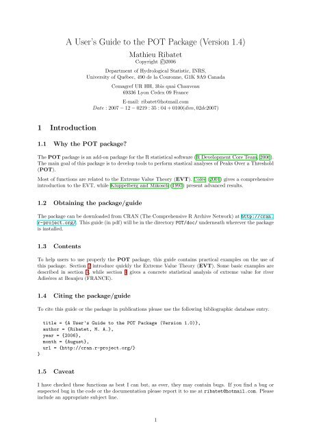
3.2 Threshold SelectionThe location for the GPD or equivalently the threshold is a particular parameter as must often it is notestimated as the other ones. All methods to define a suitable threshold use the asymptotic approximationdefined by equation (2.3). In other words, we select a threshold for which the asymptotic distribution Hin equation (2.4) is a good approximation.The POT package has several tools to define a reasonable threshold. For this purpose, the user must usetcplot, mrlplot, lmomplot, exiplot and diplot functions.The main goal of threshold selection is to selects enough events to reduce the variance; but not too muchas we could select events coming from the central part of the distribution 1 and induce bias.3.2.1 Threshold Choice plot: tcplotLet X ∼ GP (µ 0 , σ 0 , ξ 0 ). Let µ 1 be a another threshold as µ 1 > µ 0 . The random variable X|X > µ 1 isalso GPD with updated parameters σ 1 = σ 0 + ξ 0 (µ 1 − µ 0 ) and ξ 1 = ξ 0 . Letσ ∗ = σ 1 − ξ 1 µ 1 (3.1)With this new parametrization, σ ∗ is independent of µ 1 . Thus, estimates of σ ∗ and ξ 1 are constant forall µ 1 > µ 0 if µ 0 is a suitable threshold for the asymptotic approximation.Threshold choice plots represent the points defined by:where x max is the maximum of the observations x.{(µ 1 , σ ∗ ) : µ 1 ≤ x max } and {(µ 1 , ξ 1 ) : µ 1 ≤ x max } (3.2)Moreover, confidence intervals can be computed using Fisher information.Here is an application.> x par(mfrow = c(1, 2))> tcplot(x, u.range = c(0.9, 0.995))Results of the tcplot function is displayed in Figure 1. We can see clearly that a threshold around 0.98is a reasonable choice. However, in practice decision are not so clear-cut as for this synthetic example.3.2.2 Mean Residual Life Plot: mrlplotThe mean residual life plot is based on the theoretical mean of the GPD. Let X be a r.v. distributedas GP D(µ, σ, ξ). Then, theoretically we have:E [X] = µ +When ξ ≥ 1, the theoretical mean is infinite.σ , for ξ < 1 (3.3)1 − ξIn practice, if X represents excess over a threshold µ 0 , and if the approximation by a GPD is good enough,we have:E [X − µ 0 |X > µ 0 ] = σ µ 0(3.4)1 − ξFor all new threshold µ 1 such as µ 1 > µ 0 , excesses above the new threshold are also approximate by aGPD with updated parameters - see section 3.2.1. Thus,E [X − µ 1 |X > µ 1 ] = σ µ 11 − ξ = σ µ 0+ ξµ 11 − ξ(3.5)1 i.e. not extreme events.5

Modified Scale−0.2 0.0 0.2 0.4 0.6 0.8●● ● ●●●●●● ●● ● ●●●● ● ●● ●●●●●●Shape−0.8 −0.6 −0.4 −0.2 0.0 0.2●● ● ● ●● ●●●●●●●● ●● ● ●● ● ●●●●●0.90 0.94 0.980.90 0.94 0.98ThresholdThresholdFigure 1: The threshold selection using the tcplot function6

Mean Residual Life PlotMean Excess0.25 0.30 0.35 0.40 0.45 0.501.0 1.5 2.0 2.5ThresholdFigure 2: The threshold selection using the mrlplot functionThe quantity E [X − µ 1 |X > µ 1 ] is linear in µ 1 . Or, E [X − µ 1 |X > µ 1 ] is simply the mean of excessesabove the threshold µ 1 which can easily be estimated using the empirical mean.A mean residual life plot consists in representing points:{(n µ) }1 ∑µ, x i,nµ − µ : µ ≤ x maxn µi=1(3.6)where n µ is the number of observations x above the threshold µ, x i,nµ is the i-th observation above thethreshold µ and x max is the maximum of the observations x.Confidence intervals can be added to this plot as the empirical mean can be supposed to be normallydistributed (Central Limit Theorem). However, normality doesn’t hold anymore for high threshold asthere are less and less excesses. Moreover, by construction, this plot always converge to the point (x max , 0).Here is another synthetic example.> x mrlplot(x, u.range = c(1, quantile(x, probs = 0.995)), col = c("green",+ "black", "green"), nt = 200)Figure 2 displays the mean residual life plot. A threshold around 2.5 should be reasonable.7

3.2.3 L-Moments plot: lmomplotL-moments are summary statistics for probability distributions and data samples. They are analogous toordinary moments – they provide measures of location, dispersion, skewness, kurtosis, and other aspectsof the shape of probability distributions or data samples – but are computed from linear combinations ofthe ordered data values (hence the prefix L).For the GPD, the following relation holds:where τ 4 is the L-Kurtosis and τ 3 is the L-Skewness.The L-Moment plot represents points defined by:τ 4 = τ 31 + 5τ 35 + τ 3(3.7){(ˆτ 3,u , ˆτ 4,u ) : u ≤ x max } (3.8)where ˆτ 3,u and ˆτ 4,u are estimations of the L-Kurtosis and L-Skewness based on excesses over threshold uand x max is the maximum of the observations x. The theoretical curve defined by equation (3.7) is tracedas a guideline.Here is a trivial example.> x lmomplot(x, u.range = c(0.9, quantile(x, probs = 0.9)), identify = FALSE)Figure 3.2.3 displays the L-Moment plot. By passing option identiy = TRUE user can click on the graphicto identify the threshold related to the point selected.We found that this graphic has often poor performance on real data.3.2.4 Dispersion Index Plot: diplotThe Dispersion Index plot is particularly useful when dealing with time series. The EVT statesthat excesses over a threshold can be approximated by a GPD. However, the EVT also states that theoccurrences of these excesses must be represented by a Poisson process.Let X be a r.v. distributed as a Poisson distribution with parameter λ. That is:Pr [X = k] = e−λ λk, k ∈ N. (3.9)k!Thus, we have E [X] = V ar [X]. Cunnane (1979) introduced a Dispersion Index statistic defined by:DI = s2λ(3.10)where s 2 is the intensity of the Poisson process and λ the mean number of events in a block - most oftenthis is a year. Moreover, a confidence interval can be computed by using a χ 2 test:[ ]χ2(1−α)/2,M−1I α =, χ2 1−(1−α)/2,M−1(3.11)M − 1 M − 1where Pr [DI ∈ I α ] = α.For the next example, we use the data set ardieres included in the POT package. Moreover, as ardieresis a time series, and thus strongly auto-correlated, we must “extract” extreme events while preservingindependence between events. This is achieved using function clust 2 .> data(ardieres)> events diplot(events, u.range = c(2, 20))The Dispersion Index plot is presented in Figure 4. From this figure, a threshold around 5 should bereasonable.2 The clust function will be presented later in section 3.6.8

●●●L−Moments Plotτ 40.0 0.2 0.4 0.6 0.8 1.0●●● ● ●●0.0 0.2 0.4 0.6 0.8 1.0τ 3Figure 3: fig: The threshold selection using the lmomplot function9

Dispersion Index PlotDispersion Index0.8 1.0 1.2 1.4 1.6 1.85 10 15 20ThresholdFigure 4: The threshold selection using the diplot function10

3.3 Fitting the GPD3.3.1 The univariate caseThe main function to fit the GPD is called fitgpd. This is a generic function which can fit the GPDaccording several estimators. There are currently 17 estimators available: method of moments moments,maximum likelihood mle, biased and unbiased probability weighted moments pwmb, pwmu, mean powerdensity divergence mdpd, median med, pickands’ pickands, maximum penalized likelihood mple and maximumgoodness-of-fit mgf estimators. For the mgf estimator, the user has to select which goodness-of-fitstatistics must be used. These statistics are the Kolmogorov-Smirnov, Cramer von Mises, AndersonDarling and modified Anderson Darling. See the html help page of the fitgpd function to see all ofthem. Details for these estimators can be found in (Coles, 2001), (Hosking and Wallis, 1987), (Juárezand Schucany, 2004), (Peng and Welsh, 2001) and (Pickands, 1975).The MLE is a particular case as it is the only one which allows varying threshold. Moreover, two typesof standard errors are available: “expected” or “observed” information of Fisher. The option obs.fishspecifies if we want observed (obs.fish = TRUE) or expected (obs.fish = FALSE).As Pickands’ estimator is not always feasible, user must check the message of feasibility return by functionfitgpd.We give here several didactic examples.> x mom mle pwmu pwmb pickands med mdpd mple ad2r print(rbind(mom, mle, pwmu, pwmb, pickands, med, mdpd, mple,+ ad2r))scale shapemom 1.7563811022 0.21890796mle 1.7669554034 0.21254750pwmu 1.7577270679 0.21830938pwmb 1.7670734558 0.21415289pickands 1.9398703365 0.09973551med 1.9837826885 0.05076009mdpd 1.7779268149 0.20440353mple 1.7825858914 0.20187921ad2r 0.0006977949 47.80717364The MLE, MPLE and MGF estimators allow to fix either the scale or the shape parameter. For example,if we want to fit a Exponential distribution, just do (with eventually a fixed scale parameter):> x fitgpd(x, thresh = 1, shape = 0, est = "mle")Estimator: MLEDeviance: 304.1777AIC: 306.1777Varying Threshold: FALSE11

Threshold Call: 1Number Above: 100Proportion Above: 1Estimatesscale1.684Standard Error Type: observedStandard Errorsscale0.1684Asymptotic Variance Covariancescalescale 0.02834Optimization InformationConvergence: successfulFunction Evaluations: 7Gradient Evaluations: 1> fitgpd(x, thresh = 1, scale = 2, est = "mle")Estimator: MLEDeviance: 306.4435AIC: 308.4435Varying Threshold: FALSEThreshold Call: 1Number Above: 100Proportion Above: 1Estimatesshape-0.05112Standard Error Type: observedStandard Errorsshape0.06158Asymptotic Variance Covarianceshapeshape 0.003792Optimization InformationConvergence: successfulFunction Evaluations: 28Gradient Evaluations: 6If now, we want to fit a GPD with a varying threshold, just do:> x fitgpd(x, 1:2, est = "mle")12

Estimator: MLEDeviance: -173.0829AIC: -169.0829Varying Threshold: TRUEThreshold Call: 1:2Number Above: 500Proportion Above: 1Estimatesscale shape0.29079 0.06207Standard Error Type: observedStandard Errorsscale shape0.01934 0.04929Asymptotic Variance Covariancescale shapescale 0.0003739 -0.0006681shape -0.0006681 0.0024297Optimization InformationConvergence: successfulFunction Evaluations: 43Gradient Evaluations: 12Note that the varying threshold is repeated cyclically until it matches the length of object x.3.3.2 The bivariate caseThe generic function to fit bivariate POT is fitbvgpd. There is currently 6 models for the bivariateGPD - see Annexe A. All of these models are fitted using maximum likelihood estimator. Moreover, theapproach uses censored likelihood - see (Smith et al., 1997).> x y Mlog MlogCall: fitbvgpd(data = cbind(x, y), threshold = c(0, 2), model = "log")Estimator: MLEDependence Model and Strenght:Model : Logisticlim_u Pr[ X_1 > u | X_2 > u] = 0.005Deviance: 1374.676AIC: 1384.676Marginal Threshold: 0 2Marginal Number Above: 500 500Marginal Proportion Above: 1 1Joint Number Above: 500Joint Proportion Above: 1Number of events such as {Y1 > u1} U {Y2 > u2}: 50013

Estimatesscale1 shape1 scale2 shape2 alpha1.0666 0.2287 0.5332 -0.2896 0.9961Standard Errorsscale1 shape1 scale2 shape2 alpha0.07309 0.05292 0.03009 0.03676 0.02326Asymptotic Variance Covariancescale1 shape1 scale2 shape2 alphascale1 5.342e-03 -2.387e-03 9.421e-06 -7.986e-06 6.973e-06shape1 -2.387e-03 2.801e-03 -8.893e-07 5.643e-06 -4.683e-05scale2 9.421e-06 -8.893e-07 9.055e-04 -9.400e-04 2.521e-05shape2 -7.986e-06 5.643e-06 -9.400e-04 1.351e-03 -4.686e-05alpha 6.973e-06 -4.683e-05 2.521e-05 -4.686e-05 5.409e-04Optimization InformationConvergence: successfulFunction Evaluations: 71Gradient Evaluations: 19In the summary, we can see lim_u Pr[ X_1 > u | X_2 > u] = 0.02 . This is the χ statistics of Coleset al. (1999). For the parametric model, we have:χ = 2 − V (1, 1) = 2 (1 − A(0.5))For independent variables, χ = 0 while for perfect dependence, χ = 1. In our application, the value0.02 indicates that the variables are independent – which is obvious. In this perspective, it is possible tofixed some parameters. For our purpose of independence, we can run -which is equivalent to fit x and yseparately of course:> fitbvgpd(cbind(x, y), c(0, 2), model = "log", alpha = 1)Call: fitbvgpd(data = cbind(x, y), threshold = c(0, 2), model = "log", alpha = 1)Estimator: MLEDependence Model and Strenght:Model : Logisticlim_u Pr[ X_1 > u | X_2 > u] = 0Deviance: 1374.704AIC: 1382.704Marginal Threshold: 0 2Marginal Number Above: 500 500Marginal Proportion Above: 1 1Joint Number Above: 500Joint Proportion Above: 1Number of events such as {Y1 > u1} U {Y2 > u2}: 500Estimatesscale1 shape1 scale2 shape21.0667 0.2285 0.5334 -0.2899Standard Errorsscale1 shape1 scale2 shape20.07310 0.05292 0.03008 0.03672Asymptotic Variance Covariance14

Pickands' Dependence FunctionA (x)0.5 0.6 0.7 0.8 0.9 1.00.0 0.2 0.4 0.6 0.8 1.0xFigure 5: The Pickands’ dependence functionscale1 shape1 scale2 shape2scale1 5.343e-03 -2.388e-03 7.884e-14 -1.132e-13shape1 -2.388e-03 2.800e-03 1.100e-14 -1.579e-14scale2 7.884e-14 1.100e-14 9.049e-04 -9.388e-04shape2 -1.132e-13 -1.579e-14 -9.388e-04 1.348e-03Optimization InformationConvergence: successfulFunction Evaluations: 44Gradient Evaluations: 8Note that as all bivariate extreme value distributions are asymptotically dependent, the χ statistic ofColes et al. (1999) is always equal to 1.Another way to detect the strength of dependence is to plot the Pickands’ dependence function – seeFigure 5. This is simply done with the pickdep function.> pickdep(Mlog)The horizontal line corresponds to independence while the other ones corresponds to perfect dependence.Please note that by construction, the mixed and asymetric mixed models can not model perfect dependencevariables.15

3.3.3 Markov Chains for ExceedancesThe classical way to perform an analysis of peaks over a threshold is to fit the GPD to cluster maxima.However, there is a waste of data as only the cluster maxima is considered. On the contrary, if we fit theGPD to all exceedances, standard errors are underestimated as we consider independence for dependentobservations. Here is where Markov Chains can help us. The main idea is to model the dependencestructure using a Markov Chains while the joint distribution is obviously a multivariate extreme valuedistribution. This idea was first introduces by Smith et al. (1997).In the remainder of this section, we will only focus with first order Markov Chains. Thus, the likelihoodfor all exceedances is:L(y 1 , . . . , y n ; θ, ψ) =∏ ni=2 f(y i−1, y i ; θ, ψ)∏ n−1i=2 f(y i; θ)(3.12)where f(y i−1 , y i ; θ, ψ) is the joint density, f(y i ; θ) is the marginal density, θ is the marginal GPD parametersand ψ is the dependence parameter. The marginals are modelled using a GPD, while the jointdistribution is a bivariate extreme value distribution.For our application, we use the simmc function which simulate a first order Markov chain with extremevalue dependence structure.> mc mc fitmcgpd(mc, 2, "log")Call: fitmcgpd(data = mc, threshold = 2, model = "log")Estimator: MLEDependence Model and Strenght:Model : Logisticlim_u Pr[ X_1 > u | X_2 > u] = 0.611Deviance: 1702.063AIC: 1708.063Threshold Call:Number Above: 998Proportion Above: 1Estimatesscale shape alpha1.0722 0.2083 0.4739Standard Errorsscale shape alpha0.11130 0.04711 0.02243Asymptotic Variance Covariancescale shape alphascale 0.0123885 -0.0016126 -0.0013705shape -0.0016126 0.0022197 -0.0004502alpha -0.0013705 -0.0004502 0.0005030Optimization InformationConvergence: successfulFunction Evaluations: 47Gradient Evaluations: 1316

3.4 Confidence IntervalsOnce a statistical model is fitted, it is usual to gives confidence intervals. Currently, only mle, pwmu,pwmb, moments estimators can computed confidence intervals. Moreover, for method mle, “standard” and“profile” confidence intervals are available.If we want confidence intervals for the scale parameters:> x mle mom pwmb pwmu gpd.fiscale(mle, conf = 0.9)conf.inf.scale conf.sup.scale1.741236 2.493913> gpd.fiscale(mom, conf = 0.9)conf.inf.scale conf.sup.scale1.740168 2.550767> gpd.fiscale(pwmu, conf = 0.9)conf.inf.scale conf.sup.scale1.703622 2.451379> gpd.fiscale(pwmb, conf = 0.9)conf.inf.scale conf.sup.scale1.712005 2.462875For shape parameter confidence intervals, simply use function gpd.fishape instead of gpd.fiscale.Note that the fi stands for “Fisher Information”.Thus, if we want profile confidence intervals, we must use functions gpd.pfscale and gpd.pfshape. Thepf stands for “profile”. These functions are only available with a model fitted with MLE.> par(mfrow = c(1, 2))> gpd.pfscale(mle, range = c(1, 2.9), conf = 0.9)If there is some troubles try to put vert.lines = FALSE or changethe range...conf.inf conf.sup1.758081 2.525758> gpd.pfshape(mle, range = c(0, 0.6), conf = 0.85)If there is some troubles try to put vert.lines = FALSE or changethe range...conf.inf conf.sup0.01515152 0.25757576Confidence interval for quantiles - or return levels - are also available. This is achieved using: (a) theDelta method or (b) profile likelihood.17

If there is some troubles try to put vert.lines = FALSE or changethe range...conf.inf conf.sup1.758081 2.525758If there is some troubles try to put vert.lines = FALSE or changethe range...conf.inf conf.sup0.01515152 0.25757576Profile Log−likelihood−390 −385 −380 −375Profile Log−likelihood−382 −380 −378 −3761.0 1.5 2.0 2.5Scale Parameter0.0 0.2 0.4 0.6Shape ParameterFigure 6: The profile log-likelihood confidence intervals18

conf.inf conf.sup7.220334 10.219962If there is some troubles try to put vert.lines = FALSE or changethe range...conf.inf conf.sup7.50000 10.61111Profile Log−likelihood−410 −400 −390 −3806 8 10 12 14 16Return LevelFigure 7: The profile log-likelihood confidence interval for return levels> gpd.firl(pwmu, prob = 0.95)conf.inf conf.sup7.220334 10.219962> gpd.pfrl(mle, prob = 0.95, range = c(5, 16))If there is some troubles try to put vert.lines = FALSE or changethe range...conf.inf conf.sup7.50000 10.61111The profile confidence interval functions both returns the confidence interval and plot the profile loglikelihoodfunction. Figure 7 depicts the graphic window returned by function gpd.pfrl for the returnlevel associated to non exceedence probability 0.95.19

Model0.0 0.4 0.8Probability plot−● ● ●●●●●Empirical10.0 11.0QQ−plot−−−−−− − −−−−●● ●● ●●● ●● ●● ●●● ● ●−−−−−−−− −− −−●−0.0 0.2 0.4 0.6 0.8 1.0Empirical10.0 10.5 11.0 11.5 12.0ModelDensity PlotReturn Level PlotDensity0.0 0.5 1.0 1.5 2.0Return Level10.0 11.0 12.0●●●●● ●●● ●● ●●● ● ● ●10 11 12 13 14Quantile1 2 5 20 100 500Return Period (Years)Figure 8: Graphical diagnostic for a fitted POT model (univariate case)3.5 Model CheckingTo check the fitted model, users must call function plot which has a method for the uvpot, bvpot andmcpot classes. For example, this is a generic function which calls functions: pp (probability/probabilityplot), qq (quantile/quantile plot), dens (density plot) and retlev (return level plot) for the uvpot class.Here is a basic illustration of the function plot for the class uvpot.> x fitted par(mfrow = c(2, 2))> plot(fitted, npy = 1)Figure 8 displays the graphic windows obtained with the latter execution.If one is interested in only a probability/probability plot, there is two options. We can call function pp orequivalently plotgpd with the which option. The “which” option select which graph you want to plot.That is:ˆ which = 1 for a probability/probability plot;ˆ which = 2 for a quantile/quantile plot;ˆ which = 3 for a density plot;20

ˆ which = 4 for a return level plot;Note that “which” can be a vector like c(1,3) or 1:3.Thus, the following instruction gives the same graphic.> plot(fitted, which = 1)> pp(fitted)If a return level plot is asked (4 ∈ which), a value for npy is needed. “npy” corresponds to the meannumber of events per year. This is required to define the “return period”. If missing, the default value(i.e. 1) will be chosen.3.6 Declustering TechniquesIn opposition to block maxima, a peak over threshold can be problematic when dealing with time series.Indeed, as often time series are strongly auto-correlated, select naively events above a threshold may leadto dependent events.The function clust tries to identify peaks over a threshold while meeting independence criteria. For thispurpose, this function needs at least two arguments: the threshold u and a time condition for independencetim.cond. Clusters are identify as follow:1. The first exceedance initiates the first cluster;2. The first observation under the threshold u “ends” the cluster unless tim.cond does not hold;3. The next exceedance which hold tim.cond initiates a new cluster;4. The process is iterated as needed.Here is an application on flood discharges for river Ardière at Beaujeu. A preliminary study shows thattwo flood events can be considered independent if they do not lie within a 8 days window. Note that unitto define tim.cond must be the same than the data analyzed.> data(ardieres)> events clustMax rp2prob(50, 1.8)npy retper prob1 1.8 50 0.9888889> prob2rp(0.6, 2.2)npy retper prob1 2.2 1.136364 0.621

obs0 10 20 30 40● ●● ● ●● ●● ● ● ● ● ● ● ●● ● ●●● ●● ● ● ●●●●1971.5 1972.0 1972.5timFigure 9: The identified clusters. Data Ardières, u = 2, tim.cond = 822

obs0 10 20 30 401970 1975 1980 1985 1990 1995 2000 2005timeFigure 10: Instantaneous flood discharges and averaged dischaged over duration 3 days. Data ardieres3.7.2 Unbiased Sample L-Moments: samlmuThe function samlmu computes the unbiased sample L-Moments.> x samlmu(x, nmom = 5)l_1 l_2 t_3 t_4 t_50.513337801 0.167081430 -0.048173952 -0.004168153 0.0213183163.7.3 Mobile average window on time series: ts2tsdThe function ts2tsd computes an“average”time series tsd from the initial time series ts. This is achievedby using a mobile average window of length d on the initial time series.> data(ardieres)> tsd plot(ardieres, type = "l", col = "blue")> lines(tsd, col = "green")The latter execution is depicted in Figure 10.23

4 A Concrete Statistical Analysis of Peaks Over a ThresholdIn this section, we provide a full and detailed analysis of peaks over a threshold for the river Ardières atBeaujeu. Figure 10 depicts instantaneous flood discharges - blue line.As this is a time series, we must selects independent events above a threshold. First, we fix a relativelylow threshold to “extract” more events. Thus, some of them are not extreme but regular events. This isnecessary to select a reasonable threshold for the asymptotic approximation by a GPD - see section 2.> summary(ardieres)timeobsMin. :1970 Min. : 0.0221st Qu.:1981 1st Qu.: 0.236Median :1991 Median : 0.542Mean :1989 Mean : 1.0243rd Qu.:1997 3rd Qu.: 1.230Max. :2004 Max. :44.200NA's : 1.000> events0 par(mfrow = c(2, 2))> mrlplot(events0[, "obs"])> abline(v = 6, col = "green")> diplot(events0)> abline(v = 6, col = "green")> tcplot(events0[, "obs"], which = 1)> abline(v = 6, col = "green")> tcplot(events0[, "obs"], which = 2)> abline(v = 6, col = "green")From Figure 11, a threshold value of 6m 3 /s should be reasonable. The Mean residual life plot - top leftpanel- indicates that a threshold around 10m 3 /s should be adequate. However, the selected thresholdmust be low enough to have enough events above it to reduce variance while not too low as it increasethe bias 3 .Thus, we can now “re-extract” events above the threshold 6m 3 /s, obtaining object events1. This isnecessary as sometimes events1 is not equal to observations of events0 greater than 6m 3 /s. We cannow define the mean number of events per year “npy”. Note that an estimation of the extremal index isavailable.> events1 npy print(npy)[1] 1.707897> attributes(events1)$exi[1] 0.1247265Let’s fit the GPD.> mle par(mfrow = c(2, 2))> plot(mle, npy = npy)24

timeobsMin. :1970 Min. : 0.0221st Qu.:1981 1st Qu.: 0.236Median :1991 Median : 0.542Mean :1989 Mean : 1.0243rd Qu.:1997 3rd Qu.: 1.230Max. :2004 Max. :44.200NA's : 1.000Mean Residual Life PlotDispersion Index PlotMean Excess0 5 10 15 20Dispersion Index0.6 1.0 1.4 1.85 10 150 10 20 30 40ThresholdThresholdModified Scale−100 −60 −20 20●●●●●●●●●●●● ●●●● ●●●● ● ● ●●●Shape−1 1 2 3 4 5●●●●●●●●●●●● ● ●●● ●● ●● ● ● ●● ●5 10 155 10 15ThresholdThresholdFigure 11: Threshold selection for river Ardières at Beaujeu.25

−Probability plotQQ−plotModel0.0 0.4 0.8−−−−−−−−−−−−−−−−−−−−−−−−−−−−−−−−−−−−−−−−−−−−−−−−−−−−−−−−−−−−−−−−−−−−−−−−−−−−−−−−−−−−−−−−−−−−−−−−−−−−−− − −− − − −●●● ●●●●●●●●●●●●● ● ●●●●●●●● ●● ●●●●●●●●●●●● ●● ●●●●●●●●●● ● ●●●●●Empirical10 20 30 40−●● ● ●●●●● ●●●●● ●−−−−−−−−−−− − − −−−−− −−−−−●0.0 0.2 0.4 0.6 0.8 1.05 10 15 20 25 30EmpiricalModelDensity PlotReturn Level Plot●Density0.00 0.10 0.20Return Level5 15 25 35● ● ●●● ●●●●●●● ● ● ●●10 20 30 40 50Quantile0.5 2.0 5.0 20.0 100.0Return Period (Years)Figure 12: Graphic diagnostics for river Ardières at Beaujeu26

The result of function fitgpd gives the name of the estimator, if a varying threshold was used, thethreshold value, the number and the proportion of observations above the threshold, parameter estimates,standard error estimates and type, the asymptotic variance-covariance matrix and convergence diagnostic.Figure 12 shows graphic diagnostics for the fitted model. It can be seen that the fitted model “mle” seemsto be appropriate. Suppose we want to know the return level associated to the 100-year return period.> rp2prob(retper = 100, npy = npy)npy retper prob1 1.707897 100 0.9941448> prob qgpd(prob, loc = 6, scale = mle$param["scale"], shape = mle$param["shape"])scale36.44331To take into account uncertainties, Figure 13 depicts the profile confidence interval for the quantileassociated to the 100-year return period.> gpd.pfrl(mle, prob, range = c(25, 100), nrang = 200)If there is some troubles try to put vert.lines = FALSE or changethe range...conf.inf conf.sup25.56533 90.76633Sometimes it is necessary to know the estimated return period of a specified events. Lets do it with thelarger events in “events1”.> maxEvent maxEvent[1] 44.2> prob probshape0.9974115> prob2rp(prob, npy = npy)npy retper prob1 1.707897 226.1982 0.9974115Thus, the largest events that occurs in June 2000 has approximately a return period of 240 years.Maybe it is a good idea to fit the GPD with the other estimators available in the POT package.3 As the asymptotic approximation by a GPD is not accurate anymore.27

If there is some troubles try to put vert.lines = FALSE or changethe range...conf.inf conf.sup25.56533 90.76633Profile Log−likelihood−143.5 −143.0 −142.5 −142.0 −141.540 60 80 100Return LevelFigure 13: Profile-likelihood function for the 100-year return period quantile28

ADependence Models for Bivariate Extreme Value DistributionsA.1 The Logisitic modelThe logisitic model is defined by:V (x, y) =(x −1/α + y −1/α) α, 0 < α ≤ 1 (A.1)Independence is obtained when α = 1 while total dependence for α → 0.The Pickands’ dependence function for the logistic model is:A : [0, 1] −→ [0, 1][w ↦−→ (1 − w) 1 α+ w 1 α] αA.2 The Asymetric Logistic modelThe asymetric logistic model is defined by:with 0 < α ≤ 1, 0 ≤ θ 1 , θ 2 ≤ 1.V (x, y) = 1 − θ 1x+ 1 − θ 2y[ ( ) − 1 ( ) xα − 1] αyα++ ,θ 1 θ 2Independence is obtained when either α = 1, θ 1 = 0 or θ 2 = 0. Differents limits occur when θ 1 and θ 2are fixed and α = 1 → 0.The Pickands’ dependence function for the asymetric logistic model is:A(w) = (1 − θ 1 ) (1 − w) + (1 − θ 2 ) w +[(1 − w) 1 1α θα1 + w 1 1α θα2] αA.3 The Negative Logistic modelThe negative logistic model is defined by:V (x, y) = 1 x + 1 y − (xα + y α ) − 1 α, α > 0 (A.2)Independence is obtained when α → 0 while total dependence when α → +∞.The Pickands’ dependence function for the negative logistic model is:A(w) = 1 − [ (1 − w) −α + w −α] − 1 αA.4 The Asymetric Negative Logistic modelThe asymetric negative logistic model is defined by:V (x, y) = 1 x + 1 [( ) α ( ) α ] − 1x yαy − +, α > 0, 0 < θ 1 , θ 2 ≤ 1θ 1 θ 2Independence is obtained when either α → 0, θ 1 → 0 or θ 2 → 0. Different limits occur when θ 1 and θ 2are fixed and α → +∞.The Pickands’ dependence function for the asymetric negative logistic model is:[ (1 ) −α ( ) ] −α − 1α− w wA(w) = 1 −+θ 1 θ 229

A.5 The Mixed modelThe mixed model is defined by:V (x, y) = 1 x + 1 y −αx + y , 0 ≤ α ≤ 1Independence is obtained when α = 0 while total dependence could never be reached.The Pickands’ dependence function for the mixed model is:A(w) = 1 − w (1 − w) αA.6 The Asymetric Mixed modelThe asymetric mixed model is defined by:V (x, y) = 1 x + 1 y−(α + θ) x + (α + 2θ) y(x + y) 2 , α ≥ 0, α + 2θ ≤ 1, α + 3θ ≥ 0Independence is obtained when α = θ = 0 while total dependence could never be reached.The Pickands’ dependence function for the asymetric mixed model is:A(w) = θw 3 + αw 2 − (α + θ) w + 1ReferencesP. Bortot and S. Coles. The multivariate gaussian tail model: An application to oceanographic data.Journal of the Royal Statistical Society. Series C: Applied Statistics, 49(1):31–49, 2000.S. Coles. An Introduction to Statistical Modelling of Extreme Values. Springer Series in Statistics.Springers Series in Statistics, London, 2001.S. Coles, J. Heffernan, and J. Tawn. Dependence measures for extreme value analyses. Extremes, 2(4):339–365, December 1999.C. Cunnane. Note on the poisson assumption in partial duration series model. Water Resour Res, 15(2):489–494, 1979.M. Falk and R.-D. Reiss. On pickands coordinates in arbitrary dimensions. Journal of MultivariateAnalysis, 92(2):426–453, 2005.R.A. Fisher and L.H. Tippett. Limiting forms of the frequency distribution of the largest or smallestmember of a sample. In Proceedings of the Cambridge Philosophical Society, volume 24, pages 180–190,1928.J.R.M. Hosking and J.R. Wallis. Parameter and quantile estimation for the generalized pareto distribution.Technometrics, 29(3):339–349, 1987.A. F. Jenkinson. The frequency distribution of the annual maximum (or minimum) values of meteorologicalevents. Quaterly Journal of the Royal Meteorological Society, 81:158–172, 1955.S.F. Juárez and W.R. Schucany. Robust and efficient estimation for the generalized pareto distribution.Extremes, 7(3):237–251, 2004. ISSN 13861999 (ISSN).C. Klüppelberg and A. May. Bivariate extreme value distributions based on polynomial dependencefunctions. Math Methods Appl Sci, 29(12):1467–1480, 2006. ISSN 01704214 (ISSN).C. Kluppelberg and T. Mikosch. Large deviations of heavy-tailed random sums with applications ininsurance and finance. Journal of Applied Probability, 34(2):293–308, 1997.30

Liang Peng and A.H. Welsh. Robust estimation of the generalized pareto distribution. Extremes, 4(1):53–65, 2001.J. Pickands. Multivariate extreme value distributions. In Proceedings 43rd Session International StatisticalInstitute, 1981.J. III Pickands. Statistical inference using extreme order statistics. Annals of Statistics, 3:119–131, 1975.R Development Core Team. R: A Language and Environment for Statistical Computing. R Foundation forStatistical Computing, Vienna, Austria, 2006. URL http://www.R-project.org. ISBN 3-900051-07-0.S. I. Resnick. Extreme Values, Regular Variation and Point Processes. New–York: Springer–Verlag, 1987.R. L. Smith. Multivariate Threshold Methods. Kluwer, Dordrecht, 1994.R.L. Smith, J.A. Tawn, and S.G. Coles. Markov chain models for threshold exceedances. Biometrika, 84(2):249–268, 1997. ISSN 00063444 (ISSN).31