Presentation - Juha Yli-Kaakinen

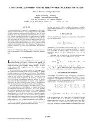
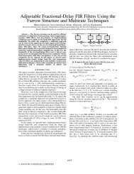
Systematic Algorithm for Designing 

Multiplierless Computationally Efficient 

Recursive Decimators and Interpolators 

Juha Yli-Kaakinen and Tapio Saramäki 

Institute of Signal Processing 

Tampere University of Technology 

Finland 

4th International Symposium on 

Image and Signal Processing and Analysis 

Yli-Kaakinen and Saramäki 

Computationally Efficient Decimators and Interpolators

Outline 

1 Recursive Decimators and Interpolators 

Introduction to Nth-band Filters 

Commutative Structures for Nth-band Filters 

Single-stage and Multistage Decimators and Interpolators 

Definition of “Multiplierless” Filters 

2 Filter Optimization 

Optimization Problem 

Optimization Algorithm 

3 Examples 

Illustrative Example 



Filter Optimization Examples Nth-band Filters Efficient structures Single- and Multistage 

Recursive Nth-band Filters 

Why Recursive Nth-band Filters? 

Best structures for decimation and interpolation: 

Low multiplication rate 

Very low sensitivity when implemented using wave digital structures 

Transfer function: 

The polyphase structure: 

H(z) = 1 N 

N−1 

∑ 

n=0 

z −n A n (z N ), 

where A n (z)’s are all-pass 

transfer functions. 

x(n) 

A 0(z N ) 

z −1 A 1(z N ) 

1/N 

y(n) 

z −2 A 2(z N ) 

z −(N−1) A N−1(z N ) 




Commutative Structures for Interpolation & Decimation 

Highly efficient structures 

A 0 (z N ) A 0 (z N ) 

x(n) 

f s 

A 1 (z) 

A 2 (z) 

1/N 

y(n) 

f s/N 

x(n) 

f s 

A 1 (z) 

A 2 (z) 

y(n) 

Nf s 

A N−1 (z) 

A N−1 (z) 

N-to-1 Decimator 

1-to-N Interpolator 

A n (z N )’s are realized at the lower sampling rate 

⇛ The computational workload is reduced by N. 




Multistage Decimators and Interpolators 

If the sampling rate conversion ratio can be factored into the product 

I∏ 

N = N i , 

where N 1 , N 2 , . . . , N I are integers, then the decimation can be 

implemented using I stages. 

Multistage Decimator 

i=1 

x(n) 

H 1 (z) N 1 H 2 (z) N 2 H I (z) N I 

y(n) 

f s f s /N 

A general implementation for an N-to-1 decimator. 

x(n) 

y(n) 

H 1 (z)H 2 (z N 1)H 3 (z N 1N 2 )· · ·H I (z N 1N 2···N I ) N 1 N 2· · ·N I 

f s 

f s /N 

Its single-stage equivalent. 




Multiplierless Filters 

Definition: “Multiplierless” filters 

Multiplication of a data sample by each coefficient value is carried out 

by using the sequence of shifts and adds (or subtracts). 

Example 

h(n) = 2 −1 − 2 −3 + 2 −5 = 0.406 25 

Desired coefficient representation form 

R∑ each a 

a r 2 −Pr 

r is 1 or −1 and 

P r ’s are integers. 

r=1 

Implementation 

2 −1 2 −3 2 −5 

Typically R is two or three 

Irregular coefficient representation form! 

PSfrag replacements 



Filter Optimization Examples Problem Algorithm 

Optimization Problem 

Statement of the problem 

Given the filter specifications 

a) the passband edge ω p , 

b) the sampling ratio alternation factor N, 

c) the number of stage I , and 

d) the stopband edge. 

Find the filter parameters 

1) the orders of the subfilters K i ’s and 

2) the discrete coefficient values 

in such a manner that 

i) the filter meets the given specifications, 

ii) the implementation cost, that is, the number of adders required to 

implement all the coefficients is minimized. 




Two-Step Optimization Algorithm 

Coefficient optimization is performed in two stages: 

Step 1: Use a nonlinear optimization algorithm for determining a 

parameter space including the feasible space where the filter 

meets the given criteria. 

Step 2: Search the filter parameters in this space in such a manner 

that the resulting filter meets the given criteria with the 

simplest coefficient representation forms. 

Property 

It has been experimentally proved that the optimum finite-wordlength 

solution can always be found. 

Particularly efficient technique for all-pass filters 

Only the denominator coefficients have to be quantized. 




Optimization Algorithm 

Step 1: Optimization of Infinite-Precision Filters 

For each filter coefficient (real pole), determine the smallest and largest 

values, denoted by 

r (n)(min) 

l 

and r (n)(max) 

l 

for l = 1, 2, . . . , K n and n = 0, 1, . . . , N − 1, 

so that by reoptimizing the values of the remaining coefficients the 

magnitude response meets the given criteria. 

Step 2: Optimization of Finite-Precision Filters 

After finding the infinite-precision search space, check whether in this 

space there exist combinations of discrete pole positions satisfying the 

specifications. 

Can be done by evaluating the magnitude response for each combination 

of discrete coefficient values between r (n)(min) 

l 

’s and r (n)(max) 

l 

’s. 



Filter Optimization Examples Illustrative Example 

Illustrative Example: Infinite-Precision Optimization 

Specifications: ω p = 0.0785π = 0.628π/8 and δ s = 0.001 (60 dB) 

Three-stage design: Cascade of three half-band filters 

The number of multipliers required to meet the specifications for 

H 3 (z 4 ), H 2 (z 2 ), and H 1 (z) are 3, 2, and 1, respectively. 

Ω s =[ 1 4 − ω p, 1 4 + ω p]∪ 

[ 1 2 − ω p, 1 2 + ω p]∪ 

0 

−10 

−20 

[ 3 4 − ω p, 3 4 + ω p]∪ 

[π − ω p , π] 

Magnitude in dB 

−30 

−40 

−50 

−60 

H 3(z 4 ) 

H 2(z 2 ) 

H 1(z) 

H 1(z)H 2(z 2 )H 3(z 4 ) 

−70 

−80 

−90 

−100 

0 

1/8π 

1/4π 

3/8π 1/2π 5/8π 

Angular Frequency ω 

3/4π 

7/8π 

π 




Illustrative Example: Finite-Precision Optimization 

The smallest and largest values for the parameters 

H 3(z 4 ) 

H 2(z 2 ) 

H 1(z) 

r (0)(min) 

1 = −0.1116 r (0)(max) 

1 = −0.0578 ∆r (0) 

1 = 0.0538 

r (0)(min) 

2 = −0.7711 r (0)(max) 

2 = −0.6811 ∆r (0) 

2 = 0.0900 

r (1)(min) 

1 = −0.3952 r (1)(max) 

1 = −0.2684 ∆r (1) 

1 = 0.1268 

r (0)(min) 

1 = −0.1568 r (0)(max) 

1 = −0.0824 ∆r (0) 

1 = 0.0744 

r (1)(min) 

1 = −0.6190 r (1)(max) 

1 = −0.4899 ∆r (1) 

1 = 0.1291 

r (0)(min) 

1 = −0.3418 r (0)(max) 

1 = −0.3366 ∆r (0) 

1 = 0.0052 

Coefficient representation: 4 power-of-two terms and 8 fractional bits 

H 3(z 4 ) 

H 2(z 2 ) 

H 1(z) 

14 discrete values between r (0)(min) 

1 and r (0)(max) 

1 



2 9702 combinations 



1 



1 

627 combinations 



1 

1 discrete value between r (0)(min) 


1 1 combination 




Quantization of H 2 (z) 

r (1) 

1 

−2 −3 

−0.1168 

r (1)(max) 

1 = −0.4899 

−0.5486 

−2 −1 − 2 −4 

r (1)(min) 

1 = −0.6190 

r (0)(min) 

1 = −0.1568 r (0)(max) 

1 = −0.0824 

r (0) 

1 

x Initial value. x optimal value. 




Illustrative Example: Optimized Coefficient Values 

The optimal finite-precision solution between the smallest and largest 

values of the coefficients 

r (0)(min) 

1 = −0.1116 < −2 −4 − 2 −6 < r (0)(max) 

1 = −0.0578 

H 3(z 4 ) r (0)(min) 

2 = −0.7711 < −1 + 2 −2 + 2 −5 + 2 −7 < r (0)(max) 

2 = −0.6811 

r (1)(min) 

1 = −0.3952 < −2 −2 − 2 −4 < r (1)(max) 

1 = −0.2684 

H 2(z 2 ) r (0)(min) 

1 = −0.1568 < −2 −3 < r (0)(max) 

1 = −0.0824 

r (1)(min) 

1 = −0.6190 < −2 −1 − 2 −4 < r (1)(max) 

1 = −0.4899 

H 1(z) r (0)(min) 

1 = −0.3418 < −2 −1 + 2 −3 + 2 −5 + 2 −8 < r (0)(max) 

1 = −0.3366 




Magnitude Response for the Optimized Three-Stage Filter 

H 1 (z) H 2 (z 2 ) H 3 (z 4 ) H 1 (z)H 2 (z 2 )H 3 (z 4 ) 

0 

−10 

−20 

Magnitude in dB 

−30 

−40 

−50 

−60 

−70 

−80 

−90 

−100 

0 

1/8π 

1/4π 

3/8π 1/2π 5/8π 

Angular Frequency ω 

3/4π 

7/8π 

π 




Pole-Zero Plot for the Optimized Three-Stage Filter 

Imaginary Part 

1 

0.8 

0.6 

0.4 

0.2 

0 

−0.2 

−0.4 

−0.6 

−0.8 

−1 

7/8π 

π 

9/8π 

3/4π 

5/4π 

5/8π 

11/8π 

2 

2 

1/2π 

3/2π 

2 3/8π 

2 

13/8π 

1/4π 

7/4π 

1/8π 

15/8π 

−1.5 −1 −0.5 0 0.5 1 1.5 

Real Part 

(b) 

7 

0 



Comparison 


Example: ω p = 0.0785π = 0.628π/8 and δ s = 0.001 (60 dB) 

Structure N M N A N O δ p δ s 

Three-stage 6 9 45 4.91 · 10 −7 0.977 · 10 −3 

Two-stage 9 8 61 1.07 · 10 −6 0.976 · 10 −3 

Single-stage 14 23 140 1.70 · 10 −6 0.979 · 10 −3 

N A give the number of adders, 

N M is the number of multipliers, and 

N O denote the overall order the filter. 

(Number of multipliers for the corresponding linear-phase three-stage 

FIR decimator when utilizing coefficient symmetry is 33.) 




Further Reading 

M. Renfors and T. Saramäki, “Recursive Nth-band digital filters 

— Part I: Design and properties, Part II: Design of multistage 

decimators and interpolators,” IEEE Trans. Circuits Syst., vol. 

CAS-34, no. 1, pp. 24–51, Jan. 1987. 

T. Saramäki and M. Renfors, “Nth-band filter design,” in Proc. 

IX European Signal Processing Conf., Island of Rhodes, Greece, 

Sept. 1998, pp. 1943–1947. 

J. Yli-Kaakinen and T. Saramäki, “Design of low-sensitivity and 

low-noise recursive digital filters using a cascade of low-order 

lattice wave digital filters,” IEEE Trans. Circuits Syst. II, vol. 46, 

pp. 906–914, July 1999. [Online]. Available: 

http://alpha.cc.tut.fi/~ylikaaki/CAS99.pdf

Presentation - Juha Yli-Kaakinen

Create successful ePaper yourself

Delete template?

Save as template?