Interactive Global Illumination Based on Coherent Surface Shadow ...

<strong>Interactive</strong> <strong>Global</strong> <strong>Illumination</strong> <strong>Based</strong> on Coherent Surface Shadow Maps
Tobias Ritschel 1 Thorsten Grosch 1 Jan Kautz 2 Hans-Peter Seidel 1
1 MPI Informatik, Saarbrücken
2 University College, London
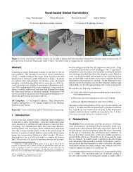
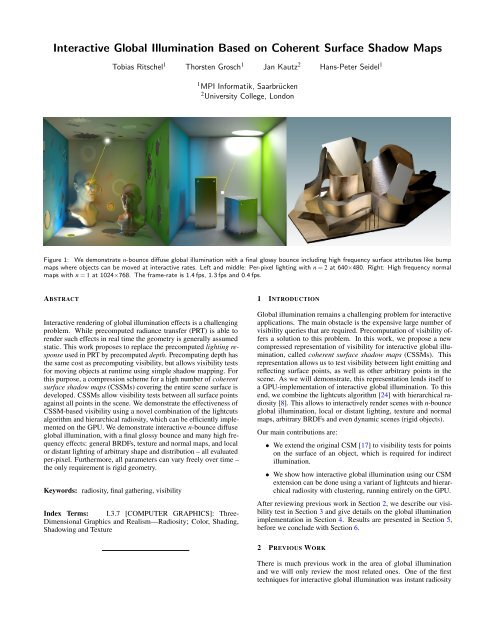
Figure 1: We demonstrate n-bounce diffuse global illumination with a final glossy bounce including high frequency surface attributes like bump
maps where objects can be moved at interactive rates. Left and middle: Per-pixel lighting with n = 2 at 640×480. Right: High frequency normal
maps with n = 1 at 1024×768. The frame-rate is 1.4 fps, 1.3 fps and 0.4 fps.
ABSTRACT
<strong>Interactive</strong> rendering of global illumination effects is a challenging
problem. While precomputed radiance transfer (PRT) is able to
render such effects in real time the geometry is generally assumed
static. This work proposes to replace the precomputed lighting response
used in PRT by precomputed depth. Precomputing depth has
the same cost as precomputing visibility, but allows visibility tests
for moving objects at runtime using simple shadow mapping. For
this purpose, a compression scheme for a high number of coherent
surface shadow maps (CSSMs) covering the entire scene surface is
developed. CSSMs allow visibility tests between all surface points
against all points in the scene. We demonstrate the effectiveness of
CSSM-based visibility using a novel combination of the lightcuts
algorithm and hierarchical radiosity, which can be efficiently implemented
on the GPU. We demonstrate interactive n-bounce diffuse
global illumination, with a final glossy bounce and many high frequency
effects: general BRDFs, texture and normal maps, and local
or distant lighting of arbitrary shape and distribution – all evaluated
per-pixel. Furthermore, all parameters can vary freely over time –
the only requirement is rigid geometry.
Keywords: radiosity, final gathering, visibility
Index Terms: I.3.7 [COMPUTER GRAPHICS]: Three-
Dimensional Graphics and Realism—Radiosity; Color, Shading,
Shadowing and Texture
1 INTRODUCTION
<strong>Global</strong> illumination remains a challenging problem for interactive
applications. The main obstacle is the expensive large number of
visibility queries that are required. Precomputation of visibility offers
a solution to this problem. In this work, we propose a new
compressed representation of visibility for interactive global illumination,
called coherent surface shadow maps (CSSMs). This
representation allows us to test visibility between light emitting and
reflecting surface points, as well as other arbitrary points in the
scene. As we will demonstrate, this representation lends itself to
a GPU-implementation of interactive global illumination. To this
end, we combine the lightcuts algorithm [24] with hierarchical radiosity
[8]. This allows to interactively render scenes with n-bounce
global illumination, local or distant lighting, texture and normal
maps, arbitrary BRDFs and even dynamic scenes (rigid objects).
Our main contributions are:
• We extend the original CSM [17] to visibility tests for points
on the surface of an object, which is required for indirect
illumination.
• We show how interactive global illumination using our CSM
extension can be done using a variant of lightcuts and hierarchical
radiosity with clustering, running entirely on the GPU.
After reviewing previous work in Section 2, we describe our visibility
test in Section 3 and give details on the global illumination
implementation in Section 4. Results are presented in Section 5,
before we conclude with Section 6.
2 PREVIOUS WORK
There is much previous work in the area of global illumination
and we will only review the most related ones. One of the first
techniques for interactive global illumination was instant radiosity

[11], where many virtual point lights (VPLs) are placed on surfaces
where indirect light is to be emitted. Rendering can then be done on
GPUs, achieving near-interactive rates. The lightcuts algorithm [24]
as well as matrix row-column sampling [9] allow illumination from
the required large number (several thousands) of VPLs in sublinear
time. The visibility test from VPLs towards the scene is an important
building block for such algorithms and two methods are available:
raytracing and shadow mapping. Raytracing for many VPLs [22]
has seen much improvement in speed over recent years on CPUs,
but its efficiency is still lacking on current GPUs. While shadow
mapping is desirable for current GPUs, it is restricted by memory
requirements and the fact that computation of shadow map pixels
that are not used to query a VPL later on is wasteful. To remedy
this, Laine et al. [13] find important VPLs (and their shadow maps)
and re-use them over time in order to compute one-bounce indirect
illumination from a single point light. Pre-computed and compressed
depth maps [17] allow visibility tests between moving objects and a
high number of lights outside their convex hulls using simple shadow
mapping, but is unsuitable for VPLs placed on an object’s surface.
Recently, several full global illumination algorithms tailored to
GPUs were proposed. Dachsbacher et al. [6] and Dong et al. [7]
demonstrate global illumination using techniques based on hierarchical
radiosity, yet avoiding traditional visibility computation. Only
per-vertex and low-frequency lighting is supported due to directional
discretization. Dachsbacher and Stamminger [5] introduce the idea
of reflective shadow maps, where shadow map texels correspond
to VPLs. However, no hierarchical lighting and no visibility were
taken into account.
The classic PRT [19] approach allows static scenes under distant
low-frequency lighting, visibility and BRDFs, which was extended
to all frequencies in [14] and other follow up work. In PRT, scenes
are usually assumed to remain static. Limited dynamic scenes (rigid
objects) can be supported, e.g. by Zhou et al. [27], but indirect
illumination is then very difficult to achieve [10][15]. This was
generalized to deforming geometry in [16]. Recently, Akerlund et
al. [1] demonstrated real-time one-bounce global illumination in
conjunction with local lighting. However, geometry still needs to be
static due the use of precomputed visibility.
In this work, we present n-bounce global illumination for dynamic
scenes consisting of several rigid objects.
3 COHERENT SURFACE SHADOW MAPS
3.1 CSM and Limitations
Coherent Shadow Maps (CSM) are a generalization of shadow maps.
Traditional shadow mapping allows visibility queries from a single
light position to all scene points. CSMs generalize this to visibility
queries between nearly all possible light positions – namely those
outside the convex hull of the scene – and all possible scene points.
At the cost of precomputation and quantization, this allows visibility
tests similar to raytracing, but without shooting any rays.
To this end, a large number of orthographic depth maps, viewing
the object from a large number of directions are precomputed and
compressed. Compression proceeds by first determining a coherent
sequence of depth maps. The sequence of depth values along each
spatial pixel is then compressed by approximating it with a piecewise
constant approximation, which can be shown to be a lossless
compression [25]. This piecewise constant approximation is then
well-suited for compression. Rendering with CSMs is similar to
traditional shadow mapping [26]. For a given scene point p on the
object, the depth map D which corresponds to the incoming light
direction is selected. The compressed depth value stored in D is
decompressed and compared to the depth of p seen from D. For
details we refer to Ritschel et al. [17].
As noted, CSMs only allow for visibility queries with light positions
outside the convex hull of the object. One example is shown in Fig. 2:
An orthographic depth map is viewing the object from outside and a
single depth value z xy is stored for this viewing direction. However,
further depth values along that ray would be required to test if the
points p i and p j are mutually visible or not. Coherent surface shadow
maps solve this issue, as will be shown in the next subsection.
q
Figure 2: Limitations of the CSM data structure: A visibility query
between the points p i and p j is not possible because only one depth
value z xy is stored for this direction in pixel q. In this example, the
required depth values between p i and p j are omitted.
z
3.2 Coherent Surface Shadow Maps
To allow lights inside the convex hull, we propose Coherent Surface
Shadow Maps (CSSM). Here, a depth cube map is swept along
the surface of the object and the depth values in all directions are
recorded. One example is shown in Fig. 3. In case of a coherent
sequence of depth cube maps, the same compression scheme used
for CSMs can be applied: An arbitrary depth value between the first
and second intersection point is stored for each pixel [25].
Different from the original CSMs, we now use depth from an inside
out perspective. This has the benefit of permitting visibility tests for
all points in any location. The challenge is to find a way to place the
depth cube maps in such a way that:
• The mesh surface has a good coverage – this allows high
frequency visibility;
• The coherence between depth maps is high – resulting in lower
memory usage and shorter decompression time
Figure 3: The CSSM stores depth values recorded from various
points on the surface of the object. Therefore, a depth cube map is
swept along the surface of the object. A few of these cube maps are
visualized on the back of the bunny.
3.2.1 Depth Cube Map Details
One half of the depth pixels of a depth cube map are in the negative
half-space and therefore contain useless depth values from inside
the object. This causes only a small amount of additional memory
because the depth value of these pixels is set to ’don’t care’ which
means that an arbitrary value can be stored here after compression.
p
p

Alternatively, a hemi-cube could be used and rotated to the tangent
frame at each surface position. We did not consider this option
because of the lower coherence of depth values for a pixel due to the
rotation of the depth cube map. To avoid depth fighting problems,
we use linear depth values [2]. In this way, we can use a small value
for the near plane without precision problems for larger depth values.
Some small surface details in front of the near plane can be lost, here
normal mapping is used to simulate them. The far plane is adjusted
to the maximum diameter of the scene.
3.2.2 Visibility Query
A visibility query works as follows (see Fig. 4): To test if the
point p i (3D position of the current fragment) is in shadow of an
arbitrary sender point p j , the depth values at p j are determined. After
projecting p i in the coordinate system of p j , the pixel position q and
the depth value z xy are known. There is an occlusion between p i and
p j if z xy is smaller than q z (the depth value of p i in the coordinate
system of p j ). Because of the discretization (depth map resolution
and cube map positions), banding artifacts can appear in shadow
regions. The same generalized percentage closer filtering (PCF)
used with CSMs can be used to improve shadow quality.
p
z
q
p
Figure 5: Illuminated atlas for the Cornell Box scene.
position. See left of Figure 6 and Figure 7 for a visualization of this
process.
The Spiral strategy moves along the border of each chart, marking
each visited texel. This can be thought of as walking along left hand
side of the border as long as possible. If there is no free texel in
the neighborhood, we step back recursively until a free neighbor
is available. Typically, this leads to a spiral-shape where texels are
visited from outside to inside. As before, a depth cube map is created
for the position associated with each texel. The right side of Figure 6
and Figure 7 show this traversal strategy.
1
1
3 3
Figure 4: CSSM visibility test: To test visibility from the point p j to
p i , we project p i into the cube map of p j giving pixel q and compare
it’s depth z xy to the depth of p i .
2
2
3.2.3 Coherent Depth Cube Maps through Atlas Traversal
Our goal is to find a sequence of depth cube maps with a minimal
amount of storage after compression. Similar to the CSM, coherence
between the depth maps is an important precondition for a
good compression. Finding a coherent sequence can therefore be
visualized as moving a depth cube map along the surface of an object
in small steps such that only small changes in the depth values occur,
thereby visiting each location of the surface exactly once. Such a
parametrization of the surface of an arbitrary complex object is not
a trivial task. A common way to parameterize the surface of an
object is to use a texture atlas, which can either be created manually
or automatically (we use Autodesk 3ds Max). The atlas is a large
texture which contains the following information for each texel: 3D
position, normal, area, radiance and BRDF parameters (eg. diffuse
color, roughness, glossiness).
An atlas consists of so-called charts describing connected regions
of the object (see Fig. 5 for an example). Moving from one texel to
its neighbour is likely to be coherent if we stay inside a chart. We
therefore avoid to simply visit all texels inside the atlas, and instead
develop two strategies for a coherent traversal where one chart after
the other is visited: Zig-Zag and Spiral.
For the Zig-Zag strategy we first determine the bounding box of the
(first) chart. We then visit all texels inside the box in a zig-zag pattern
from top to bottom. For each texel, we retrieve the corresponding 3D
position and generate a depth cube map for it. If a texel is undefined
(or belongs to a different chart), we skip it. After visiting all texels
of one chart, we move to the next chart which has the closest 3D
Figure 6: Coherent traversal in an atlas with three charts: A traversal
strategy is used for each chart. Left: Zig-Zag. Right: Spiral.
Figure 7: Traversing the Cornell box (left: zig-zag, right: spiral)
and the Cornell Church with a depth cube map in a coherent order.
Resolution is artificially low to make the path more visible.
We do not use the Hilbert pattern (used for CSM traversal) because it
is not suited for arbitrary shaped charts. If there is no parametrization
available, we resort to a traversal that greedily walks a number of
random samples that were distributed evenly across the surface.
3.3 Moving Objects
In the case of moving objects, each object contains its own CSSM
and an additional CSM. After a rigid transformation, the same visibility
test as described in Sec. 3.2.2 can still be performed for two
points on the same object. To test if there is an occluder between

two points p i and p j located on different objects, each object uses its
own CSSM to check for self-occlusions first. There is an occlusion
between the two points p i and p j if one of the two depth tests reports
a self-occlusion. In case of no self-occlusion, all other objects must
be tested as possible occluders between p i and p j . This kind of
visibility test cannot be performed with the CSSM. Here the CSM is
required, because the visibility of an arbitrary ray can be computed
(without knowing any point on the object). So the CSM of each
additional object is used to test if the ray, starting from p i in direction
towards p j is blocked by this object. Recall that the CSM cannot
compute visibility between two points inside an object, so both data
structures are required.
Visibility tests with moving objects are possible as long as the convex
hulls of the individual objects do not overlap. Otherwise, the depth
information stored in the CSSM can become invalid because objects
might be placed at a smaller distance than the depth values stored in
the CSSM.
To enable a GPU implementation we allow only a refinement of the
sender, the receiver is always a leaf. The Refine function is therefore
a loop over all leaves in the tree and the appropriate sender levels
are computed for each leaf (this corresponds to a cut through the
tree). Because of this limitation, the PushPull function simplifies to
a Pull function to compute the radiosity values of the internal nodes.
Fig. 8 shows a simple example of our GPU HRC algorithm.
Repeat
Compute Cut Gather Pull
4 GLOBAL ILLUMINATION
The original CSM data structure allows visibility tests for arbitrary
direct illumination (point lights, area lights or environment maps)
but any emitter has to be outside the convex hull of the object
(Fig. 2), making the original CSMs unsuitable for computing indirect
illumination. In contrast, the new CSSM allows visibility tests
between arbitrary points within an object, as described in Sec. 3.2.2.
This enables the computation of additional indirect bounces of light
with correct occlusion. In this section, we describe how advanced
lighting can be computed using CSSMs, including direct lighting,
an arbitrary number of diffuse indirect bounces and a final glossy
bounce towards the viewer.
Our basic idea is to compute indirect bounces by illuminating the
atlas [3]. Here, geometric information and material data are available
for each texel and therefore each texel in the atlas represents a small
patch. A simple solution would be to use each texel as a sender, like
in GPU progressive refinement radiosity [4]. Since this is too slow
for complex scenes, we used a clustering approach.
Our lighting simulation consists of two steps:
• A GPU version of hierarchical radiosity with clustering (HRC)
to compute an arbitrary number of diffuse bounces. Here,
texels in the atlas are illuminated.
• A GPU version of final gathering including glossy materials
based on lightcuts. Here, pixels in the framebuffer are illuminated.
Figure 8: One iteration of GPU HRC for a simple scene. The leaf
nodes in the tree correspond to texels in the atlas. We assume that all
nodes already contain the direct light. For refinement, the appropriate
sender levels are selected for each receiver leaf - this results in a cut
through the hierarchy (left). Now, the receiver leaf node gathers
from all nodes of the cut (middle). For simplification, the example
shows the cut and the gather links for only one leaf. After gathering,
some red and green color bleeding is visible in the leaves. Finally, a
consistent hierarchy is restored with a pull operation (right).
4.2 Hierarchy
Given an atlas with a 3D position for each texel, an implicit hierarchy
is given by building a MIP map which stores at each texel the extent
of the spatial locations of all child-texels in the finer mip map levels.
However, we observed that this does not lead to a good hierarchy
because texels from different charts, located at completely different
spatial positions, will be combined at a certain level. Instead, we
build a separate binary tree based on a standard median cut algorithm.
To allow a fast computation of upper bounds for light transmission
during refinement, a hierarchy of bounding spheres over the original
3D points is created as well (see Fig. 9). This hierarchy is computed
as a pre-process, as neither the atlas nor the texels’ spatial locations
change at run-time, since we assume rigid objects.
4.1 Hierarchical Radiosity
The original algorithm for hierarchical radiosity [8] with clustering
[21][18] consists of three steps, repeated until convergence: Refine,
Gather and PushPull. The Refine step recursively subdivides the
self-link of the root node depending on an oracle function. The
Gather step then computes the received radiosity for each node
by summing the contribution of all links arriving at the node. In
the PushPull step, a consistent hierarchy is established by adding
the radiosities from top to bottom and computing area-weighted
averages bottom-up.
4.1.1 Hierarchical Radiosity on the GPU
A direct implementation of hierarchical radiosity on a GPU is difficult,
especially because of the Refine function, which establishes
links between arbitrary levels of senders and receivers, thereby recursively
traversing both source and receiver tree simultaneously.
Figure 9: The bottom levels of the bounding sphere hierarchy.
4.2.1 Hierarchy on the GPU
This binary tree is stored as a linear array for fast, stack-less traversal.
For each node N, we store two pointers: a child- and a skip-pointer
[20]. The child-pointer points to the left child. The skip-pointer
points to the next node for depth-first traversal, if the subtree below
N should be skipped. These two pointers are sufficient for a depthfirst
traversal: Starting from the root, always use the child-pointer

until a leaf is reached; then use the skip-pointer and continue. Moreover,
this enables a selective traversal (required for refinement), as
described in the next subsection.
For each node, all data is stored in 128 bits using a single 32-bit
RGBA integer texel. 24 bits are used for: Center position, average
normal and radiant intensity, 8 bits for: radius, normal cone angle
and area, and 16 bits for both pointers. Due to the size limitations of
one-dimensional textures, the hierarchy is stored in a native layout
as a two-dimensional texture. Both pointers are converted into this
layout when storing the hierarchy. One example is shown in the left
of Fig. 11.
4.3 Hierarchy Traversal
The data structure introduced in the previous section enables a combined
implementation of Refine and Gather for a receiver leaf node
N r : Starting from the root, the tree is traversed in depth-first order
by following the child-pointer as long as an oracle function decides
to refine the current sender node N s . In case of no refinement, N s
is an appropriate sender level and the radiance transmission from
N s to N r is computed and accumulated. To accomplish this, a form
factor and a CSSM-based visibility value are computed here. Now,
all nodes below N s can be ignored by following the skip-pointer,
and the process can be repeated. The pseudo-code for this traversal
is shown in Fig. 10.
We use an energy-based refinement oracle which computes an upper
bound of the received radiance L max from N s to N r . The same upper
bound computation as presented in [24] is used here. Now, N s is
refined if the tone-mapped value of L max is above a user-defined
threshold. In this way, the refinement adapts to the current display
settings (we use a simple gamma tone mapper in our examples).
senderNode = root
L = 0
while(senderNode != NULL) {
if oracle(senderNode, receiverNode, threshold) {
senderNode = senderNode.leftChild // Refine
}
else {
L += computeRadiance(senderNode, receiverNode)
senderNode = senderNode.skip // Gather
}
}
Figure 10: Pseudocode for stack-less GPU tree traversal. This
combines the Refine and Gather step for an arbitrary receiver leaf
node. No links need to be stored in this way.
4.4 Final Gathering
The direct visualization of a radiosity solution suffers from discretization
artifacts, like jagged shadows. Better, but slower results
are obtained when using final gathering for display. Recently, Walter
et al. [24] introduced lightcuts, a fast final gathering method. Their
original algorithm assumes a converged lighting simulation from
which a hierarchy of VPLs is created. To select the minimal number
of VPLs for a given receiver point, an initial cut through the hierarchy
is computed (usually just the root node). Then the node inside
the cut with the largest error relative to the total incident radiance
is selected. If this relative error is perceivable for the human eye
(this means larger than two percent due to Weber’s law) the node is
removed and its children are placed into the cut. This is repeated
until the node with the largest contribution is below two percent or a
maximum number of nodes is reached.
Figure 11: The glossy Cornell Box and the corresponding VPL tree
which stores direct light in a texture (left). The indirect light is
computed by final gathering. The cut size (number of nodes in the
cut) for gathering indirect light is visualized on the right.
4.4.1 Final Gathering on the GPU
We found the original lightcuts algorithm unsuitable for a GPU
implementation for two reasons. First, it requires a priority queue to
quickly identify the node with the largest error, which is difficult to
maintain efficiently on a GPU. Secondly, the original error bound is
quite expensive to compute.
Instead, we propose to construct a simplified cut for an arbitrary
receiver point: After computing multiple diffuse bounces, all nodes
in the hierarchy are VPLs which contain direct and indirect light.
Therefore, the same algorithm as shown in Fig. 10 can be used to
compute the cut and gather from all nodes in the cut. The only
difference is, that the receiver node has to be replaced by the receiver
position of the current framebuffer pixel. Because the final bounce
allows glossy surfaces, the oracle function now includes the computation
of an upper bound of the Phong BRDF [24] for computing
L max . This approach poses no constraints on the final receiver pixel
at all. We are free to use normal maps, high frequency textures and
arbitrary BRDFs. Fig. 11 (right) shows a visualization of the cut
size we achieve: For large regions in the image, a low number of
VPLs is sufficient for a good quality. A direct visualization of the
illuminated atlas is possible, but better visual results are obtained
with final gathering, as shown in Fig 17.
In comparison with the original lightcuts alorithm, we use an energybased
oracle instead of a perceptually-based criterion. Nonetheless,
we found that for a GPU implementation, the benefits of the simplifications
outweigh the algorithmic deficiencies. Recently, Akerlund
et al. also used cuts [1] for global illumination. However, they precompute
the entire cut for static vertices, whereas we find the cuts
dynamically for each pixel.
4.5 Jittering
One problem of VPL-based global illumination is the limitation to
moderately glossy BRDFs. When glossiness is increased, single
highlights become apparent where a continuous highlight should
appear. We mitigate these artifacts in our approach by associating
an approximate area with every VPL from which we pick a random
location instead of the VPL’s center location. When several frames
with different random location samples are averaged this ’VPL bias’
can be removed as can be seen in Fig. 12.

in our examples, the direct lighting is computed from spotlights with
shadow maps.
Figure 12: A highly glossy Cornell Box without jittering showing
VPL bias (left). The jittered image (middle) takes 20 s to converge.
The right image shows the absolute difference.
4.6 Discretization Artifacts
Like in all sampling-based approaches, aliasing is a central problem.
Our visibility computation has two possible sources of aliasing: The
spatial discretization due to the atlas and the limited resolution of the
depth cube maps. Fig. 13 demonstrates the visual effect of different
resolutions of the atlas. Fig. 14 shows the difference if the CSSM
visibility test is replaced by an exact ray query to the VPL. Note
that the error introduced due to the depth cube map discretization
(6 × 64 × 64) is hard to perceive, the banding artifacts appear due to
the discretization of the atlas (64 × 64).
Indirect Light Monte Carlo rendering with importance sampling
[17] can also be used for the computation of indirect bounces instead
of using HRC. Here, the atlas with the direct light serves as a
probability density function where samples are taken with a probability
proportional to the atlas texel radiance. In combination with
progressive rendering, this leads to a solution that runs at interactive
rates and converges to the correct solution if the camera is not moving.
However, importance sampling solely based on radiance does
not take distance or occlusion into account. Consequently, many
samples are taken from distant or invisible regions, resulting in a
very slow convergence. Therefore, we prefer hierarchical radiosity
for indirect lighting.
Instant Radiosity Using an atlas to compute indirect light transport
can be seen as covering the entire surface with small lambertian
area lights. This is different to reflective shadow maps [5], where
individual pixels in a projective texture from the light’s point of view
are used. <strong>Illumination</strong> atlases enables the use of general direct lighting,
which may not come from a single point light, and also allows
for more than one-bounce indirect illumination. Just like in classic
radiosity [8], the illumination atlas corresponds to a discretization of
the scene surfaces but without the overhead of meshing and is thus
more amenable to a GPU implementation. Our method can also be
interpreted in terms of instant radiosity [11]: We fix a large number
of VPLs on the surface beforehand, so we can precompute CSSMs
and enable fast visibility queries for them.
Figure 13:
Increasing the resolution of the atlas reduces banding.
5 RESULTS
We demonstrate our approach for different scenes, as shown in the
accompanying video. The system used is an Intel Core 2 Duo 6300
with 2 GB RAM and an NVIDIA GeForce 8800.
Speed We measured the performance of our visibility test, and
found that it performs well around 150M samples per second (lighting
computations from a VPL including visibility). Tbl. 1 shows a
list of the measured performance.
Figure 14: Comparison: Visibility using raytracing (left) and CSSMs
(center). The right image shows the absolute difference. Two forms
of artifacts can be seen for CSSMs, which are both original shadow
mapping problems. First, limited spatial resolution makes shadow
edges appear jagged. Secondly, limited depth quantization and spatial
resolution requires to use a depth bias which never works for all
shadow maps at the same time.
4.7 Discussion
Several alternatives exist for implementing global illumination:
Direct Light The computation of direct lighting can be separated
from the computation of indirect lighting. For direct illumination,
any method that generates physically plausible direct lighting can
be used, e.g. the Monte-Carlo based illumination for light sources
outside the convex hull of the scene, used for the original CSM [17].
After direct illumination the inner nodes of the hierarchy can be
filled with a pull operation and the following indirect bounces can be
computed with the GPU HRC simulation. We did not use this option
Table 1: Frame rates for different number of indirect bounces.
The column ’samples’ lists screen pixels or atlas texels of the viewdependent
lightmap. In all cases, the direct lighting runs with more
than 100 fps.
Cornell
Box
Cornell
Heads
Cornell
Church
Scene Samples Bounces fps
640×480 1 5.2 fps
Pixels 2 1.4 fps
128×128 1 35.7 fps
Texels 2 10.4 fps
640×480 1 7.4 fps
Pixels 2 1.3 fps
128×128 1 7.8 fps
Texels 2 4.0 fps
640×480 1 4.1 fps
Pixels 2 0.7 fps
128×128 1 11.9 fps
Texels 2 3.1 fps
Compression We found the CSSMs compress nearly as good
as CSMs, which means one or two orders of magnitude of data
compression (Tbl. 3). Tbl. 2 shows a comparison between different
traversal strategies. The Cornell Church scene achieves a compression
ratio of up to 21.4 : 1, although it is a difficult case: Due to

Table 2: Compression factors for a Cornell box with 6×32×32 depth
map resolution, different atlas resolutions and traversal strategies. A
simple greedy strategy is always worse than the chart-based traversals.
Spiral slightly outperforms Zig-Zag.
Atlas Res.
Strategy
Greedy Zig-Zag Spiral
32×32 5.6 : 1 7.1 : 1 7.4 : 1
64×64 8.8 : 1 11.2 : 1 11.7 : 1
128×128 12.8 : 1 15.7 : 1 16.9 : 1
many parallax events and the high genus, there is low coherency
in depth. The best compression ratio is 41.5 : 1, enabling several
gigabytes of depth data. It is impossible to render such a high number
of depth maps dynamically or store them uncompressed with
current GPUs. This can be seen from the fact that the compression
time is dominated by rendering the depth maps alone (doubling the
resolution nearly doubles time). Therefore dynamically rendering
this many shadow maps would take time in the same order as the
precomputation — many minutes.
Quality
To verify the correctness of our GPU HRC algorithm, we compare
our solution with pbrt (Fig. 15). Except of the discretization artifacts,
the radiance distribution is the same. Fig. 16 shows the illumination
with a varying number of bounces. As explained, we are not limited
to vertex lighting which is a bandlimitation of the lighting and
prevents pixel exact convergence. Vertex-based global illumination
techniques mostly use ten-thousands of vertices which is one order
of magnitude less than the hundred-thousands of samples used in
this work. Note that we select only a small fraction of them for
each screen pixel individually (the cut), enabling a glossy bounce
at interactive frame rates. To avoid VPL-based artifacts at short
distances, clamping is used which can lead to darkening of edges.
For comparison to other work, we include performance for viewdependent
lightmapping, see Tbl. 1 and Fig. 17, where the resulting
indirect lighting is computed for every atlas texel and not every pixel
in the frame-buffer; only the direct lighting contribution is computed
at every frame buffer pixel. We use a high quality bicubic texture
filter in order to prevent mach-banding, e.g., at shadow edges.
Figure 15: The radiance distribution of our solution (left) is nearly
identical to a solution computed with pbrt (right).
6 CONCLUSIONS
In this work, a visibility test for interactive global illumination
based on pre-computed depth was presented. The key feature of
our approach is its generality; besides rigid object transformations
and non-overlapping convex hulls for moving objects, no further
constraints are imposed. This allows many effects required for high
Figure 17: Left: Final Gathering. Right: Direct visualization of the
atlas with a final, glossy bounce computed for each atlas texel. The
atlas is identical to the one used for the CSSM. Although indirect
lighting itself is smooth, some sharp features are visible, like the text
on the floor and the reflection from the right head back to the left
one. The textures are 2 k×2 k in size and do not tile which would
result in at least 4 M vertices when converted to geometry.
quality rendering at interactive rates: Hierarchical radiosity with
per-pixel lighting and normal mapping to name a few examples that
are difficult to produce with other methods.
As future work, we want to investigate if a complete dynamic hierarchical
radiosity is possible on the GPU, including an arbitrary
receiver level and better refinement oracles. Moreover, we would
like to research light transport not only between final screen pixels
and the scene, but between groups of pixels and the scene, mixing
hierarchical radiosity and irradiance caching [12]. Using nonlambertian
VPLs by fitting multiple Phong lobes [23] appears as
another promising avenue of further research. A combination of
the CSM data structure with depth peeling would be one possible
approach to remove the convex hull restriction of moving objects.
Ultimately, we would like to remove all the remaining constraints
on scene configuration and rigid objects.
REFERENCES
[1] O. Akerlund, M. Unger, and R. Wang. Precomputed Visibility Cuts
for <strong>Interactive</strong> Relighting with Dynamic BRDFs. Proceedings Pacific
Graphics 2007, 2007. 2, 5
[2] S. Brabec, T. Annen, and H.-P. Seidel. Practical Shadow Mapping.
Journal of Graphics Tools, 7(4):9–18, 2002. 3
[3] N. Carr, J. Hall, and J. Hart. GPU Algorithms for Radiosity and
Subsurface Scattering. In Graphics Hardware 2003, pages 51–59, July
2003. 4
[4] G. Coombe, M. J. Harris, and A. Lastra. Radiosity on graphics hardware.
In Proceedings of Graphics Interface 2004, pages 161–168,
School of Computer Science, University of Waterloo, Waterloo, Ontario,
Canada, 2004. Canadian HC Communications Society. 4
[5] C. Dachsbacher and M. Stamminger. Reflective Shadow Maps. In
Proceedings of the ACM SIGGRAPH 2005 Symposium on <strong>Interactive</strong>
3D Graphics and Games, pages 203–213, 2005. 2, 6
[6] C. Dachsbacher, M. Stamminger, G. Drettakis, and F. Durand. Implicit
Visibility and Antiradiance for <strong>Interactive</strong> <strong>Global</strong> <strong>Illumination</strong>. ACM
Trans. Graph. (Proceedings of ACM SIGGRAPH 2007), 26(3), 2007. 2
[7] Z. Dong, J. Kautz, C. Theobalt, and H.-P. Seidel. <strong>Interactive</strong> <strong>Global</strong> <strong>Illumination</strong>
Using Implicit Visibility. In Pacific Conference on Computer
Graphics and Applications, 2007. 2
[8] P. Hanrahan, D. Salzman, and L. Aupperle. A Rapid Hierarchical
Radiosity Algorithm. Computer Graphics (Proceedings of ACM SIG-
GRAPH 91), 25(4):197–206, 1991. 1, 4, 6
[9] M. Hašan, F. Pellacini, and K. Bala. Matrix Row-Column Sampling for
the Many-Light Problem. ACM Trans. Graph. (Proceedings of ACM
SIGGRAPH 2007), 26(3):26, 2007. 2

Table 3: Compression rates for different objects with depth cube map resolution 6 × 64 × 64. The number of depth maps is
lower than the number of atlas texels, because some texels are undefined.
Cornell
Box
Cornell
Heads
Cornell
Church
Scene Atlas Res. Depth Maps Uncompressed Compressed Ratio Time
64×64 2592 127.4 MB 8.0 MB 15.9 : 1 43 s
34
128×128 10701 525.9 MB 21.5 MB 24.4 : 1 3 min.
Faces
256×256 42226 2.0 GB 62.1 MB 33.4 : 1 13 min.
512×512 170770 8.4 GB 202 MB 41.5 : 1 55 min.
19k
Faces
3700
Faces
64×64 2002 98.4 MB 10.1 MB 9.6 : 1 52 s
128×128 8367 411.2 GB 40.7 MB 10.1 : 1 5 min.
256×256 32964 1.6 GB 120.2 MB 13.5 : 1 18 min.
512×512 129599 6.3 GB 249.9 MB 25.4 : 1 64 min
64×64 2479 121.9 MB 34.8 MB 3.5 : 1 47 s
128×128 9869 485.1 GB 81.7 MB 5.9 : 1 4 min.
256×256 39751 2.1 GB 173.0 MB 11.3 : 1 14 min.
512×512 158969 2.1 GB (91 MB) 1 (21.4 : 1) 1 73 min.
1 Note: Current GPUs can address 8192 2 two-dimensional texels, which is often less than the available total memory. For this CSSM more than 8192 2
texels would be required. We revert to 6 × 32 × 32 depth cube maps in this case.
Figure 16:
Direct light (left, 100 fps), one indirect bounce (middle, 7.4 fps) and two indirect bounces (right, 1.4 fps).
[10] K. Iwasaki, Y. Dobashi, F. Yoshimoto, and T. Nishita. Precomputed
Radiance Transfer for Dynamic Scenes Taking into Account Light Interreflection.
In Proceedings of Eurographics Symposium on Rendering
2007, pages 35–44, 2007. 2
[11] A. Keller. Instant Radiosity. In SIGGRAPH 97: Proceedings of the 24th
annual conference on Computer graphics and interactive techniques,
pages 49–56, 1997. 2, 6
[12] J. Křivánek, K. Bouatouch, S. N. Pattanaik, and J. Žára. Making radiance
and irradiance caching practical: Adaptive caching and neighbor
clamping. In Rendering Techniques 2006, Eurographics Symposium
on Rendering, June 2006. 7
[13] S. Laine, H. Saransaari, J. Kontkanen, J. Lehtinen, and T. Aila. Incremental
Instant Radiosity for Real-Time Indirect <strong>Illumination</strong>. In
Proceedings of Eurographics Symposium on Rendering 2007, pages
277–286, 2007. 2
[14] R. Ng, R. Ramamoorthi, and P. Hanrahan. Triple Product Wavelet Integrals
for All-Frequency Relighting. ACM Trans. Graph. (Proceedings
ACM SIGGRAPH 2004), 23(3):477–487, Aug. 2004. 2
[15] M. Pan, R. Wang, X. Liu, Q. Peng, and H. Bao. Precomputed radiance
transfer field for rendering interreflections in dynamic scenes.
Computer Graphics Forum, 26(3):485–493, Sept. 2007. 2
[16] Z. Ren, R. Wang, J. Snyder, K. Zhou, X. Liu, B. Sun, P.-P. Sloan,
H. Bao, Q. Peng, and B. Guo. Real-Time Soft Shadows in Dynamic
Scenes using Spherical Harmonic Exponentiation. ACM Trans. Graph.
(Proceedings ACM SIGGRAPH 2006), 25(3):977–986, 2006. 2
[17] T. Ritschel, T. Grosch, J. Kautz, and S. Müller. <strong>Interactive</strong> <strong>Illumination</strong>
with Coherent Shadow Maps. In Proceedings of Eurographics
Symposium on Rendering 2007, pages 61–72, 2007. 1, 2, 6
[18] F. Sillion. A unified hierarchical algorithm for global illumination with
scattering volumes and object clusters. IEEE TVCG, 1(3), 1995. 4
[19] P.-P. Sloan, J. Kautz, and J. Snyder. Precomputed Radiance Transfer
for Real-time Rendering in Dynamic, Low-frequency Lighting Environments.
Proc. of ACM SIGGRAPH 2002, 21(3):527–536. 2
[20] B. Smits. Efficiency issues for ray tracing. Journal of Graphics Tools:
JGT, 3(2):1–14, 1998. 4
[21] B. Smits, J. Arvo, and D. Greenberg. A Clustering Algorithm for
Radiosity in Complex Environments. Computer Graphics, 28(Annual
Conference Series):435–442, 1994. 4
[22] I. Wald, T. Kollig, C. Benthin, A. Keller, and P. Slusallek. <strong>Interactive</strong>
<strong>Global</strong> <strong>Illumination</strong> Using Fast Ray-tracing. In Proceedings of the 13th
Eurographics workshop on Rendering, pages 15–24, 2002. 2
[23] B. Walter, G. Alppay, E. Lafortune, S. Fernandez, and D. P. Greenberg.
Fitting Virtual Lights for Non-diffuse Walkthroughs. Computer
Graphics, (Annual Conference Series):45–48, 1997. 7
[24] B. Walter, S. Fernandez, A. Arbree, K. Bala, M. Donikian, and D. P.
Greenberg. Lightcuts: A Scalable Approach to <strong>Illumination</strong>. ACM
Trans. Graph. (Proceedings of ACM SIGGRAPH 2005), 24(3):1098–
1107, 2005. 1, 2, 5
[25] D. Weiskopf and T. Ertl. Shadow Mapping <strong>Based</strong> on Dual Depth
Layers. In Eurographics 2003 Short Papers, pages 53–60, 2003. 2
[26] L. Williams. Casting Curved Shadows on Curved Surfaces. In Computer
Graphics (Proceedings of ACM SIGGRAPH 78), pages 270–274,
August 1978. 2
[27] K. Zhou, Y. Hu, S. Lin, B. Guo, and H.-Y. Shum. Precomputed Shadow
Fields for Dynamic Scenes. ACM Trans. Graph. (Proceedings ACM
SIGGRAPH 2005), 24(3):1196–1201, 2005. 2