Two-dimensional spectroscopy. Application to nuclear magnetic ...

Two-dimensional spectroscopy. Application to nuclear magnetic 

resonance 

W. P. Aue, E. Bartholdi, and R. R. Ernst 

Laboratorium fiir physikalische Chemie, Eidgeniissische Technische Hochschule, 8006 Ziirich, Switzerland 

(Received 13 November 1975) 

The possibilities for the extension of spectroscopy to two dimensions are discussed. Applications to nuclear 

magnetic resonance are described. The basic theory of two-dimensional spectroscopy is developed. 

Numerous possible applications are mentioned and some of them treated in detail, including the elucidation 

of energy level diagrams, the observation of multiple quantum transitions, and the recording of highresolution 

spectra in inhomogenous magnetic fields. Experimental results are presented for some simple 

spin systems. 

I. INTRODUCTION 

Spectroscopy in its classical form has been developed 

to investigate and to identify molecular systems in their 

linear approximation. Linearity is a crucial condition 

for the spectrum to uniquely represent the input/output 

relations of a physical system. It is particularly well 

fulfilled in optical spectroscopy as long as the use of 

lasers is disregarded. For linear systems, the entire 

apparatus of electronic sY!'tem theory1 can be employed 

to describe the methods of spectroscopy. Of particular 

importance is the equivalence of the notions "spectrum" 

and "transfer function" or "frequency response function, 

" on one hand, and of "interferogram" or "free induction 

decay" and "impulse response," on the other. 

These correspondences proved to be fruitful in connection 

with the introduction of Fourier spectroscopy in 

optical spectroscopy2 and in magnetic resonance. 3,4 

It is well known that linearity is merely an abstract 

concept to simplify the mathematical treatment. It 

does not correspond to physical reality, although it may 

be an excellent approximation, in many cases. 

In radio frequency spectroscopy, linearity is restricted 

to very weak perturbations of the investigated 

system, and nonlinear effects are well known to occur 

in almost any spectroscopic radio frequency experiment. 

Typical effects are saturation effects, line 

broadening, and line shifts caused by strong perturbations. 

5 

Some properties of molecular systems can only be 

noticed through nonlinear effects, e. g., spin-lattice 

relaxation and the connectivity of the various transitions 

in the energy level scheme. Spectroscopy has, 

therefore, been extended to include methods suitable 

for the investigation of nonlinear properties of molecular 

systems. 

A straightforward extension of spectroscopy is the 

measurement of saturation curves and the analysis of 

line shapes under the influence of strong rf fields, although, 

in most cases, the information cannot be obtained 

directly but must be extracted by means of 

iterative approximation procedures. 6 

The most fruitful class of techniques was certainly 

provided by double resonance. 7 ,8 Here, a strong perturbation 

serves to modify the system in a nonlinear 

fashion. The actual spectroscopic experiment, using 

a second, weak perturbation, can again be considered 

as the investigation of a linear system. Of particular 

importance for the elucidation of the topology of energy 

level schemes and indirectly of molecular structure are 

techniques like spin tickling, 9 INOOR, 10 and selective 

population transfer. 11 

Another class of experiments aimed towards the investigation 

of nonlinear phenomena, particularly of 

relaxation mechanisms, is formed by pulse experiments 

which have been developed into a large variety of 

techniques of great practical importance. 3,12,13 

All these methods have been devised to measure 

specific properties connected with some nonlinear behavior 

of systems. In this paper, a very general class 

of techniques will be described which is suitable for a 

much wider characterization of nonlinear properties. 

Many of the earlier techniques are contained as special 

cases. 

For the description of the nonlinear properties, it is 

not sufficient to consider just amplitude, perhaps including 

phase, as a function of frequency as it is done 

in classical spectroscopy. It is necessary to include 

at least one further parameter such as rf field strength, 

time, or a second frequency as is done, for example, 

in double resonance. 8 A graphic representation of such 

a set of data naturally leads to two-dimensional or, 

more generally, to multidimensional spectroscopy. 

In the following, we will call a two-dimensional (or 

multidimensional) plot of spectral data a "two-dimensional 

(or multidimensional) spectrum" only when all 

variables of the plotted function are frequencies, in 

contrast, for example, to stacking, in a two-dimensional 

manner, a set of spectra as a function of time as 

is frequently done in relaxation time measurements. 13 

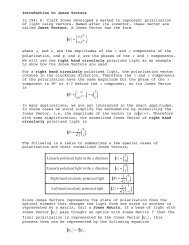
Many possibilities to generate 2D spectra are conceivable. 

Some basic schemes are shown in Fig. 1. 

(a) Frequency space experiment. The simultaneous 

application of two frequencies and measuring the response 

as a function of both frequencies leads directly 

to a 2D spectrum. This is the prinCiple of conventional 

double resonance. 8 An example of a 2 D tickling 

spectrum of the triplet of 1,1, 2-trichloroethane is 

shown in Fig. 2. A complicated pattern of ridges of 

The Journal of Chemical Physics, Vol. 64, No.5, 1 March 1976 

Copyright © 1976 American Institute of Physics 2229

2230 Aue, Bartholdi, and Ernst: Two-dimensional spectroscopy 

b c d 

S(tl. W2) S ( tl. t2) s (t) 

l' 'J'2 (21 

PRE~RATORYI 

EVOlUTK>N 

PERIOD : PERIOD 

I 

DETECTION 

PERIOD 

"3(.(2) 

I "3(.(1) I 

----~9~----~¢~---------- 

R ('1:'1 • '["2) 

y:2 

S(Wl'~) 

FIG. 3. Partitionirig of the time axis in a 2D FTS experiment. 

a 

FIG. 1. Basic schemes to n.easure and compute 2D spectra. 

fJ =Fourier transformation, e = crosscorrelation. 

changing amplitudes results. In addition, the pattern is 

strongly dependent on the rf field strength used. 

(b) Mixed frequency space time space experiment. 

A system perturbed by a strong rf field with frequency 

Wz can be investigated by applying an rf pulse and measuring 

its response. Fourier transformation of the 

free induction decay and repetition of the experiment 

for various perturbing frequencies leads also to a 2D 

spectrum with properties very similar to those of conventional 

double resonance. a ,1S 

(c) Time space experiment. A 2D experiment done 

completely in time space requires two independent time 

variables as a function of which a signal amplitude can 

be measured. A 2D Fourier transformation of the 2D 

time Signal produces then again a 2D spectrum. 16,17 

(d) Stochastic resonance experiment. From the response 

of a nonlinear system to a Gaussian random perturbation, 

it is also possible to compute a 2D spectrum 

by calculating higher cross-correlation functiOns between 

input and output noise and Fourier transforming 

them. 18 

It is not intended to give a complete survey of all 

possibilities to create 2D spectra. This paper will be 

limited to the analysis of time space experiments which 

FIG. 2. Proton resonance 2D tickling spectrum of 1,1,2- 

trichloroethane. The doublet is irradiated at various freq uencies 

w2; Wt is swept through the triplet part of the spectrum. A 

related 2D FTS spectrum is shown in Fig. 15. 

appear to be particularly fruitful. They are also of 

conceptual interest as they are generalizations of wellknown 

pulse experiments and exhibit the essential features 

of these experiments in a particularly clear way. 

Section II gives a brief survey of some possibilities 

of 2D spectroscopy. The general theory of the basic 

experiment is described in Sec. III. Considerable simplifications 

are obtained by the restriction to weakly 

coupled systems. This is shown in Sec. IV. As an 

example of a strongly coupled spin system, the twospin 

system is treated in Sec. V. Section VI is devoted 

to the phenomena in systems including equivalent spins, 

and Sec. VII describes the interesting features of 2D 

spectroscopy in the presence of inhomogeneous magnetic 

fields. Methods to observe zero quantum and double 

quantum transitions are treated in Sec. VIII. A 

few experimental aspects are mentioned in Sec. IX, 

although details on data processing in two dimensions 

and further applications will be described at another 

place. 

It should be emphasized at this point that this work 

was stimulated by a presentation of Professor Jean 

Jeener at the Ampere International Summer School II, 

Basko Polje (1971), who mentioned the idea of the twopulse 

version of 2D spectroscopy. The first experiments 

in Jeener's group were performed later by 

Alewaeters. 16 

II. TWO-DIMENSIONAL FOURIER SPECTROSCOPY 

In 2D FTS, the 2D spectrum is obtained by Fourier 

transforming a signal s(t 1 , t) which depends on two independent 

time variables t1 and t 2 • For the introduction 

of two time variables, it is necessary to mark out 

two points on the time axis and to partition the experiment 

time into three periods. For the present purpose, 

it is convenient to let t1 be the duration of the second 

period and t2 the running time in the third period, as 

shown in Fig. 3. The signal s(t 1 , t 2 ) is then measured 

in the third period as a function of t2 with t1 as a parameter. 

The three phases which are characteristic for all 2D 

FTS experiments are named according to their physical 

significance: 

t < 0; Preparation period. The system is prepared 

in a suitable initial state, described by the density operator 

u(O). 

J. Chem. Phys., Vol. 64, No.5, 1 March 1976

a) 

b) 

c) 

I 

d) 

e) 

I 

I 

tl 

·1 

Aue, Bartholdi, and Ernst: Two-dimensional spectroscopy 2231 

~ 

E I 

hv 

rf 

E 

FIG. 4. Some homonuclear schemes' for 2D FTS. (a) Basic 

two-pulse experiment. (b) Observation of Torrey oscillations. 

(c) Detection of a nonequilibrium state. (d) Fourier zeugmatography. 

(e) Detection of transient oscillations in CIDNP. 

o < t < t1: Evolution period. The system evolves under 

the influence of the Hamiltonian Je U ) and assumes 

at the end of this interval a particular state which depends 

on Je(l) and on the elapsed time fl' 

t1 < t: Detection period. The system develops further 

under the influence of the Hamiltonian Je(2). During 

this time, the transverse magnetization My(t1' t 2 ) 

= s(t1> t 2 ) is detected as a function of t 2 • 

: 

t 

In the experiment shown in Fig. 4(b), an rf field is 

applied during the evolution period. Separate preparation 

and mixing pulses are not required. During the 

evolution period, Torrey oscillations will develop. 

They can be associated with the various resonance transitions. 

A modification of this experiment, adding a 

magnetic field gradient during the detection period, may 

serve as a means to measure the spatial inhomogeneity 

of the rf field strength. 

Figure 4(c) shows an experiment where a nonequilibrium 

state a(O) is created during the preparatory 

period. The first two pulses applied permit the population 

of all matrix elements of the density operator. 

The behavior during evolution and detection periods 

then completely characterizes the initial nonequilibrium 

state. Here, 2D spectroscopy is a means to measure 

the instantaneous state a(O) of a perturbed system, including 

the matrix elements responsible for the higher 

order transitions. An example of this experiment is 

analyzed in Sec. VIII. 

Fourier zeugmatography may be considered as a 

speCial case of 2D (or 3D) spectroscopy.19 Figure 4(d) 

shows a preparatory pulse which generates the required 

transverse magnetization which precesses during the 

following time periods in the presence of two different 

magnetic field gradients. lt permits measurement of 

the 2D or 3D spatial spin density of macroscopiC (biological) 

objects. 

Nonequilibrium states can also be created by nonmagnetic 

perturbations, for example, by initiating a 

chemical reaction by means of a light pulse at time f = O. 

Figure 4(e) indicates an experiment which has been 

A large number of experiments for different duration 

t1 of the evolution period have to be performed to obtain 

a sufficiently dense sampling of the 2D time function 

s(t 1 , t 2 ). In a multidimensional extension of 2D 

spectroscopy, the system has to go through several 

evolution periods, each of which must be varied systematically 

in its length. 

a) 

s 

: 

Many homo- and heteronuclear experiments are possible 

which conform to this general scheme. Some possibilities 

are shown in Figs. 4 and 5. The basic experiment, 

suggested by Jeener, 16 is the two-pulse experiment 

of Fig. 4(a). The preparatory phase ends with a 

nonselective rf pulse at time t= 0 (called preparatory 

pulse). A flip angle of 90° is usually employed to generate 

off-diagonal elements of the density operator 

which evolve under the influence of the Hamiltonian 

Je(l) during the evolution period. This period is ended 

by a second rf field (called mixing pulse) at time t= t 1 • 

lt mixes the various magnetization components and enables 

their measurement during the detection period. 

This experiment permits elucidation of the energy level 

schemes of coupled spin systems. A very Simple application 

is also the distinction of resonance lines belonging 

to different molecules in a mixture. A detailed 

analysis of this experiment is given in Sec. m. 

b) 

c) 

s 

s 

FIG. 5. Some heteronuclear schemes for 2D FTS. The S 

magnetization is observed. (a) 2D-resolved carbon-13 resonance. 

(b) Transitory cross polarization in solids. (c) Heteronuclear 

two-pulse experiment. 

J. Chern. Phys., Vol. 64, No.5, 1 March 1976


used to measure off-diagonal elements of the density 

operator a(O) created during the chemical reaction in 

chemically induced dynamic nuclear polarization. zo 

The heteronuclear experiment shown in Fig. 5(a) 

leads to 2D-resolved carbon-13 spectroscopy, a promising 

method to unravel complicated undecoupled carbon-13 

spectra. During the evolution period, the 13C 

spins precess in the absence of proton-carbon couplings 

while the complete Hamiltonian determines the 

evolution during the detection period. This permits 

separation of the multiplets which originate from different 

carbon spins. Zl 

Figure 5(b) shows a typical cross-polarization experiment 

used in solids to detect rare nuclei. zz The 

evolution period here is identical with the cross-polarization 

time. During this period, transient oscillations 

have recently been observed. They are caused 

by the coherent dipolar interaction of directly bound 

nuclei. a3 A 2D representation of these phenomena permits 

one to obtain structural information on solid samples, 

for single crystals as well as for powders. An 

interesting modification of this technique has recently 

been developed by Waugh. a4 

Figure 5(c), finally, sketches an experiment which is 

a heteronuclear modification of the basic two pulse experiment. 

It permits one to unravel the multiplet structure 

of heteronuclear spin systems. Many more modifications 

are conceivable involving pulsed and continuous 

rf fields, optical irradiations, magnetic field gradients 

or field jumps, and other perturbations leading 

to two- or multidimensional spectra. 

In all these experiments, a 2D Fourier transformation 

is required to generate the desired complex 2D 

spectrum S(Wl' wz): 

S(Wl' wa) = fa'" dt 1 exp(- iWltl) 10'" dtz[exp(- iwztZ)]s(th ta) • 

It may be considered as a sum of four terms: 

S(w h 

w a ) = S CC(Wl' w z ) - S ""(Wh wz) 

with, e. g., 

SCC(Wh Wz)=l'" dt 1 coS(W 1 t 1 ) 1'" dtz[cos(Wzfz)]s(thta)' (3) 

o 0 

In many cases, it is more convenient to plot one of the 

four real components scc(wt> wz), S""(wt> wz), SC"(whwa), 

or S"'C(w h w a ) instead of real or imaginary part of 

S(Wl' wal. SCC(Wh wz) can be considered as a four 

quadrant average of S(W l 

, wa): 

S CC(Wh wz) = t {S(Wh wa) + S(Wl' - wa) + S(- WI' wz) 

(1) 

+ S(- wi> - wz)} • (4) 

The following symmetry relations can easily be verified 

S(- WI, - wa) = S(Wh wz)* , 

SCC(_ Wh wa) = SCC(w h - wz) = Scc(_ wt> - wa) 

= SCC(Wh wa) , 

- SSS(_ WI, wa) = - S SS(Wi> - w z ) = S8S(_ wt> - wa) 

= SS8(W h wa) , (5) 

- SSC(_ WI, wz) = S sC(w h 

- w z ) = - S 8C(_ WI' - wa) 

= SSC(Wi> wa) , 

Scs(_ WI, w z ) = - scs(w l , - w a ) = - SC8(_ WI' - w a ) 

= S CS(Wl' wz) • 

In many applications, it is sufficient to compute the 

absolute value of S(wh w z ) instead of plotting one of the 

phase sensitive components, e. g., S CC(w l , w a ). The 

absolute value spectrum is much less critical to adjustment, 

but clearly, it contains less information. 

The absolute value spectrum I S I (w h w a ) will be defined 

in the following particular manner: 

lsi (wh wa)=HI S(wt> wa)la+ I S(Wl' - wa)la 

+ I S(- WI, wz)lz+ 15(- w h - wa)lz]1/a. (6) 

This definition has the advantage that the contributions 

from all four quadrants will be taken into account, for, 

in some cases, peaks may contribute to two of the four 

quadrants only. Taking the absolute value spectrum, 

it is sufficient to plot one quadrant only. It can easily 

be shown that 

I S I (WI' wa) = [S CC(Wh wz)a + 5 C8(Wh wz)Z + S 8c(Wl' wz)a 

This equation is important for the numerical evaluation 

of experimental data. 

III. THEORETICAL DESCRIPTION OF 2D FTS 

In this section, a general 2D FTS experiment will be 

analyzed. At time t=O, the system is assumed to be 

prepared in a state described by the density operator 

a(O). It can be an arbitrary nonequilibrium state. zo 

During the time interval 0 < t < tt> the system develops 

freely under the influence of the time-independent Hamiltonian 

Jew. At time t = t l 

, the density operator is rotated 

by an rf pulse, represented by a superoperator Z5 

R. In special cases, this rf pulse may be absent [e. go, 

Figs. 4(b), 4(d), 5(a), and 5(b)]. During the remaining 

time, t> t l , the system develops freely under the timeindependent 

Hamiltonian Je(a). In many cases, Jew = Je(Z) 

[e. g., Figs. 4(a), 4(c), 4(e), and 5(c)]. In certain 

cases :Je(!) and Je(Z) can also represent time-independent 

Hamiltonians in a rotating frame [e. g., Figs. 4(b) and 

5(b) ]. 

The motion of the system is described by the density 

operator equation 

u = - i[Je(t), a] - r{a - ao(t}} , (8) 

with 

Je(l) for 0 < t < t 

Je(t) = 1 

{ 

Je(2) for t > t l 

, measured in frequency units. 

Je(!) and Je(Z) are assumed to be high field Hamiltonians. 

The equilibrium density operator ao may be different 

in the two time intervals, 


Aue. Bartholdi. and Ernst: Two-dimensional spectroscopy 2233 

u o (1) for 0 < t < t 1 , 

uo(t) = { 

(a) 

u 0 for t > t1 • 

A 

r is the relaxation superoperator. 

In a shorthand superoperator notation, a5 Eq. (8) can 

be written as 

with 

(9) 

(10) 

JC(t)u = [JC(t) , u] • 

This notation permits a straightforward solution for the 

density operator u(t h ta) at time t= t1 + ta: 

(a) (. ~ (2) ~ 

U 

( 

th ta 

) 

= Uo + exp - tJC ta - rta) 

X[~{U~ll + exp(- i~ (llt 1 

- rt 1 

)(u(0) - U6 1l )}- uc?)] . 

(11) 

The observed magnetization component, e. g., My(thta), 

is then given by 

My(t1' ta) = NylfTr[F yu(th ta)] 

.. .. .. 

= NytiTr[Fy exp(- iJC(2)t a - rt a )R{U6 1 ) 

~ '" 

+ exp(- iJC(1)t 1 - rt 1 )[u(0) - (6 1 )]} ] • (12) 

N is the number of spi~ systeIps per unit volume. The 

terms uc?) and exp(- iJC(2)t a - rt a )U6 a ) usually do not contribute 

to the observed magnetization and have been 

neglected in Eq. (12). The 2D spectrum S(w h wa) is 

finally obtained by a 2D Fourier transformation of 

My(t1' ta), 

S(W1' wa)= l~ dt 1 e-lw1t1J~ dtae-IW~aMy(th t a ) • (13) 

o 0 

For the explicit evaluation, it proves to be convenient 

to separate My(t1' ta) into the parts originating from the 

diagonal and off-diagonal parts of u(O), respectively. 

"Diagonal" and "off-diagonal" refer here to the Hamiltonian 

JCCll which is assumed to possess nondegenerate 

eigenvalues. This separation can be effected 

by means of a pair of projection superoperators with 

the properties 

1> :: 

d+n=1, 

3a=3 , ~a=~ 

dJC(1) = JC U ) , 

~ 

[dA,JC U )] = 0 for any operator A. 

One obtains 

with 

and 

My(t1' ta) = M yd(t1' ta) + M~(th ta) , 

M~(th ta) = .lV;ilfTr(Fy exp(- i:k(2)t a - f.ta)R 

x exp (- tJC 

." U) 

t1 - rt 

'" ~ ( )] 1 fTlU 0 . 

M~(t1' ta) comprises those components which show an 

(14) 

(15) 

(16) 

(17) 

AXIAL PEAK 

(@) 

FIG. 6. Schematic representation of the features of a 2D 

spectrum. 

oscillatory behavior during the evolution period. They 

will, finally, be responsible for cross peaks and dia 

peaks in the 2D spectrum (see Fig. 6). These components 

contain the .information which relates various 

transitions and which permits one to trace out the energy 

level diagram. ~(tl' t.), on the other hand, represents 

magnetization components which remain longitudinal 

during the evolution period and which do not oscillate 

during this time interval. M~(tl' ta) produces the 

axial peaks and provides information on spin-lattice 

relaxation processes. 

A. Off-diagonal elements of u(O) 

In the absence of almost degenerate transitions and 

of partially Clverlapping lines, it is possible to neglect 

all parts of r which do not commute with X. It is, 

therefore, assumed that 

[Xu>, r]=[:k(a), r]=o. (18) 

Taking into account that the relaxation superoperator 

f (represented, e. g., by the Redfield relaxation matr~6) 

is a symmetric superoperator, i. e. , 

:: .. 

Tr{AtrB} = Tr{(rA)tB} , (19) 

one obtains 

M~(tl' ta)= NyliTr{[exp(i:k(2)t a - rta)Fy] 

It ~ ~ *: 

XR[exp(- iJC(1)t 1 - rt1);iu(0)]} • 

In explicit notation, M~(th ta) is given by 

M~(tl' ta) = Nylf L L [F y/ll exp(iw~~)t2 - ta/Ta~I)] 

III ttl" 

with 

W!> = JC.!.t,,: - JC.:!) , 

w~) =~:) -JCF,) • 

, 

(20) 



In the absence of overlapping lines, each transition 

possesses a single relaxation time T2k1" The matrix 

elements of Fy are computed in the eigenbase of JC(2), 

whereas the matrix elements of ~a(O» are evaluated 

in the eigenbase ., of JCC1l. The matrix elements of the 

superoperator R are, therefore, calculated in a mixed 

base. This is indi


utilizing the property Zkl,mn=Z,tnm' The virtue of Eq. 

(31) is that, for proper phase adjustment, only one term 

remains, so that peaks with a pure phase can be obtained. 

For phase adjustment, it is necessary to form 

linear combinations of S~cIlCmnl> Sil,BIlCmn )' S(i,"IlCmn), and 

S;:,cll Cmn)' 

The absolute signal amplitudes [compare Eq. (6)], 

given by 

I Z I kl,mn = ~[I zkI,mnl 2 + I Zkl,nml 2 + I Z lk,mnl 2 + I Z'k,nmI2]1/2, 

(33) 

can also be expressed by the real amplitudes ACkI)(mn), 

..• ,D CkIl Cmn): 

I Z I kl,mn = [A~kl)(mn) + ifCkI)(mn) + C~IlCmn) + D~1l (mn)]1/2 • 

Two different kinds of. peaks can be distinguished 

which originate from Skl,mn(Wl' w2) (see Fig. 6): 

(34) 

(i) Cross peaks: they occur for (kl) '" (mn) and correlate 

different transitions. These are the "off-diagonal" 

peaks in a 2D spectrum; and 

(ii) Dia peaks: they occur for (kl) = (mn) and are related 

to one single transition, only. They occur on the 

main diagonal of the 2D spectrum. 

Cross and dia peaks contain three kinds of information: 

(a) Information about the connec tivity of transitions 

in the energy level diagram. This information is 

analogous to the one obtained from double resonance, 

particularly from tickling exp~riments. 9 It is provided 

by the rotation superoperator R which couples the various 

transitions. Particularly informative is also the 

flip angle dependence of intensities and phases. 2D 

spectra contain a wealth of information on the topology 

of the energy level diagram; 

(b) Information on transverse relaxation processes. 

The line shapes are determined by the transverse relaxation 

times T 2kl • As will be shown later, they can 

also be determined even in the presence of field inhomogeneity 

broadening; 

(c) Information on the initial state a(O) of the spin 

system. In conventional spectroscopy, allowed transitions 

can be detected only. In 2D FTS, on the other 

hand, it is possible to measure all matrix elements of 

a(O) in a unique manner. Particularly, it is possible 

to observe matrix elements responsible for zero-, 

double- and multiple-quanta transitions. This will be 

shown in Sec. VIII. 

B. Diagonal elements of a(O) 

The contributions of the M~(th t 2 ) term, which leads 

to the axial peaks, will now be evaluated in a similar 

manner. With Eq. (18), one obtains from Eq. (16) 

M ~(th t2) = Nyli L L [F yk I exp(iw:~) t2 - t21 T 2k I )]R:~~~m 

kI m 

Here, the diagonal elements of the density operator in 

the eigenbase of X (1 ) have been identified with the population 

numbers P n : 

Pn(O)=ann(O),pon=a~!~, (37) 

and W is the Redfield relaxation matrix 26 which describes 

the longitudinal relaxation in a coupled nuclear 

spin system with 

The matrix elements of exp(- Wt 1 ) can be expressed by 

the eigenvalues wJ of W: 

(38) 

[exp(- Wt1)]mn = L SmJ S:J exp(- w J t1) , (39) 

. J 

with S representing the diagonalizing transformation of 

w. 

M ~(tl' t2) will now be split into the various contributions 

to particular resonance peaks: 

with 

and 

(40) 

M ~kl(tl' t2) = Gki exp(iwk~)t2 - t21T 2k1) , (41) 

M~',J(tl' t2) = Gkl,J exp(iw:~)t2 - t2IT2kI ) exp(- wA). (42) 

The coefficients are given by 

Gu = NyliF yk I L R~~~mPom 

m 

Gkl,J = NyliFYkl L 

m 

LR~~~mSmJS.t(Pn(O) - pan) • 

n 

(43) 

Equation (41) shows that M: kI (t 1 , t 2 ) is independent of fl' 

To obtain a nondiverging Fourier integral, it is therefore 

necessary to limit the integration to 0 < f1 < fm 

where fm is a suitable upper limit for f 1 : Then, one 

obtains 

SkI,j(W1, W2)=Gkl,J{ak~)(w2)- id:~>(W2)}{WJ/{~+z0) 

-iw/{wf+wm· 

(44) 

Of particular interest is again the 2D cosine transform 

of M~(tl' t2). Here, one obtains the following contributions 

S(i.Cn(Wh W2) = [Re{Gkl}{ak~)(w2) + a::> (w 2 )} 

and in explicit matrix notation 

(35) 

- 1m {GkIH- d~>(w2)+d::>(w2)} ] 

1 . 

x - slnw1tm , 

W1 

(45) 



S Q.1),j(Wl> w2) = [Re {Gkl,j}{a~~) (w2) + a:~)(w2)} 

- 1m {GkI,J}{- d:~)(w2)+d:;)(w2)}] 

x~ . (46) 

WI +Wj 

Equations (45) and (46) describe contributions to the 2D 

spectrum which all lie on the W2 axis (WI = 0). These 

peaks are called axial peaks (see Fig. 6). Each allowed 

transition Wk~) is represented by a peak which itself 

is a superposition of Lorentzians with half-width 

Wj in the WI direction and which also contains a contribution 

proportional to (1/ w1) sinw1tm' The line shape, 

therefore, contains uT 1 " information although, particularly 

in complicated spin systems, it may be difficult 

to be extracted. 

The complete 2D spectrum is finally obtained as a 

sum of the contributions from Eqs. (31), (45), and (46): 

x[cos!a]2N-dlm-dknW/-Mk)(Mn-Mm) , (51) 

for pairs of allowed transitions (kl) and (mn). By 

means of Eq. (32), it is finally possible to compute the 

real amplitudes A(kl)(mn)"" ,D(kl)(mn)' It is seen from 

Eq. (51) that Zkl,mn is either real or imaginary. Therefore, 

two of the real amplitudes are necessarily zero. 

For transitions with aM=±l, Zkl,mn is found to be real 

and C(kl)(mn) =D{kl) (mn) =0. 

For the amplitudes Gkl and Gkl,J of the longitudinal 

contributions, one obtains Similarly 

and 

G kl = - i Q 0 

2 m 

L (- 1)dlm(i)dlm+dkm [sin!a]dlm+dkm 

x[cos!a]2N-dlm-dkmMm(MI_ M k ) , (52) 

x[cos!a]2N-dlm-dknSmJS:iMn(MI- M k ) • (53) 

+ L LS~ClljWl' w 2 ) • (47) 

(kll J 

The first term describes the cross and dia peaks, 

whereas second and third terms contribute to the axial 

peaks. 

IV. WEAKLY COUPLED HOMONUCLEAR SYSTEMS 

For weak coupling among N nonequivalent spins !, 

it is possible to derive closed expressions for intensities 

and phases in a 2D spectrum. This case provides 

an instructive insight into the features of 2D spectroscopy. 

To simplify the Situation, it is assumed that 

the initial state u(O) is prepared by means of a 90; 

pulse acting on a system in thermodynamic equilibrium. 

This produces the initial state 

(0) 

_1 + (nW~kT)Fy 

u - Tr I} . 

Additionally, JC(2) is set equal to JC(1} • Then, one obtains 

for the complex signal amplitude Zkl,mn with Eqs. 

(22), (23), and (27) 

(48) 

Nyn 2 w 

Zkl,mn = Q. FYklR ImRtnFymn with Q = kTTr{l}' (49) 

For spin !, the matrix elements FYkl are given by 

!i(MI- Mk) for allowed transitions with a 

~ 

single spin flipping, ams=± 1 

FYkl = 

and am r 

= 0 for r* s 

o for all forbidden transitions. 

Here, M/ is the magnetic quantum number of state l, 

and the matrix elements of the rotation operator Rare 

found to be 20 (50) 

whereo aIm' the spin flip number, is the number of spins 

with different spin polarization in the two states 1 and 

m. With Eqs. (49) and (50), one obtains for Zk/,mn 

To obtain a better understanding of the complex amplitudes 

Zkl,mn [Eq. (51)] it is convenient to introduce 

connectivity classes to distinguish various pairs of 

transitions. 

For a general description of connectivity in weakly 

coupled spin systems, it is necessary to indicate all 

spin states for the two transitions in question. The 

following notation is used here: (1) the two transitions 

in question are indicated by the letter of the flipping 

spin. To identify the particular transition, the lower 

magnetic quantum number of the two connected states 

is indicated by a subscript. For nonequivalent spins 

!, no indexing is required; (2) within brackets, the 

states of all other spins are indicated by their magnetic 

quantum numbers. For nonequivalent spins !, + and 

- are used to fix the spin state; and (3) for magnetically 

equivalent nuclei, the group spin quantum number 

(irreducible representation of the permutation group) 

is indicated additionally by a superscript. 

Some examples are: 

(1) 4 nonequivalent spins !: 

[A(B+C..nJ, B

a 

b 

c 

'-I / /,,-m 

A // 

//6km=5-1 

k--/ 

'T 


Tn 

only on S and on the connectivity character, and are 

given by the following values: 

Connection ~Im ~kn ~km ~/n 

Tn 

k-------+---m 

6km= 5-2 

FIG. 7. Definitions of connectivity classes for nonequivalent 

spins!. (a) Parallel pair, two A spin transitions; along the 

broken line S-1 spins ('" A) change their polarization. (b) Regressive 

pair, one A and one B spin transition; along the 

broken line S-2 spins ('" A ,B) change their polarization. (c) 

Progressive pair, one A and one B spin transition; along the 

broken line, S-2 spins ("'A,B) change their polarization. 

same polarization in the inner brackets: 

e. g., [A(B.C.DJ, B(A.CJ).)] ; 

(c) Progressive pairs: two different spins A and B 

flip in the two transitions, A and B appear with different 

polarization in the inner braCkets: 

Regressive and progressive connectivity reduce to the 

former notion when the transitions are directly connected. 

For indirectly connected transitions, regressive 

and progressive pairs are defined such that the 

elimination of all spins which do not flip in either transition 

reduces the pair to a directly connected regressive 

or progressive pair, respectively. 

A convenient shorthand notation considers only (1) the 

number of spins S necessary to describe a certain connection 

(disregarding spins which neither flip nor have 

different polarization in the two transitions); (2) the 

connectivity character (l = parallel, r = regressive, p 

= progressive); and (3) the total number of coupled 

spins. Examples are: 

[A(B.C.DJ,A(B_C.D.)]-3l4, 

[A (B. C.DJ , B(A.CJ).)] - 4 r 4 , 

[A(B.C.DJ, B(A_C_DJJ- 3p4 • 

This is the entire information which is necessary to 

compute peak intensities in a 2D spectrum, or, in 

other words, it is all the information which can be obtained 

from a 2D spectrum. 

The spin flip numbers ~Im used in Eq. (50) depend 

parallel S 5 5-1 5-1 

regressive 5-1 5-1 

progressive 

{or ~- 2 

{or ~- 2 

5- 2 

5 

S- 2 S-1 S-1 

5 

These values can easily be checked by inspection of 

Fig. 7. A distinction of the two cases indicated for 

both regressive and progressive pairs is immaterial 

since the same signal amplitudes will result in both 

cases. 

This leads, finally, to the following simple relations 

for the complex signal amplitudes Zkl,mn, and for the 

real amplitudes A(kJ)(mn) and B{kn(mn) used in Eq. (31) 

(C (kJ) (mn) = D(kn (mn) = 0 for Single quantum transitions): 

(a) Parallel pairs (S l N): 

Zkl,mn = - tQ(sin~a)2S (cos~a)2N-2S , 

Z Ik,mn = tQ(sin~a)2S-2(cos~a)2N-2s.2 , 

Aa.n (mn) = iQ(sin~a)2S-2(cos~a)2N-2Scosa , 

Ba.n (mn) = - iQ(sin~a)2S-2(cos~a)2N-2S 

(b) Regressive pairs (Sr N): 

Z = _ .!.Q(sin.!.a)2S-2(cos.!.a)2N-2S.2 

A 

kl,mn 4 2 2 , 

• 

= - .!.Q(sin.!.a)2S-2(cos.!.a\2N-2s.2 

a.1)(mn) 4 2 2 , , 

B{kl)(mn) =0 • 

(c) Progressive pairs (SpN): 

(54) 

(55) 

(56) 

(57) 

Same expressions as for regressive pairs with opposite 

sign: 

A{kn (mn) = tQ(sin~a)2S-2(cos~a)2N-2s.2 , 

(58) 

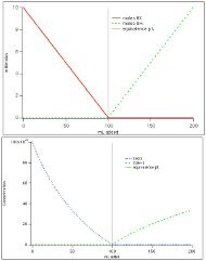
For illustration of Eqs. (54)- (58), amplitude and 

phase for the various transitions of a four-spin system 

are given in Fig. 8 as functions of the flip angle a of 

the mixing pulse. The phase is defined here as 

tan = B{kn (mn,! Aa.J) (mn) , 

and describes the mixing between pure 2D absorption 

and 2D dispersion signals. The following conclusions 

about the general behavior of 2D spectra for weakly 

coupled spin ~ systems can be drawn: 

(1) The phase of peaks caused by regressive and 

progressive pairs is independent of the flip angle a. 

Regressive and progressive pairs have opposite sign; 

(2) The phase of parallel pairs is dependent on the 

flip angle, changing by 90 0 for a variation of a from 0 0 

to 180 0 • All parallel pairs have the same phase; 

(3) For a = 0 0 , only Il N peaks have a nonvanishing 

intensity. Cross peaks are absent for a=Oo; 



180· - - - - - - 

r 

.14 

.12 

w 

C 

:;:) .10 

~ 

::::i 

Q. 

~ .08 


FIG. 9. Theoretical 2D FT spectrum of a two-spin system applying two 90° pulses to the system in equilibrium. The parameter 

values used correspond to the proton resonance of 2, 3-dibromothiophene at 60 MHz. The weak coupling assumption was not used. 

v. 2D FTS FOR A STRONGL Y COUPLED TWO-SPIN 

SYSTEM 

The matrix representations of the two operators Fy 

and R in the eigenbase of the Hamiltonian are 

In this section, explicit results will be given for a 

strongly coupled two-spin 'system and compared with 

experimental results. It is ass}lmed that the initial 

state u(O) is generated by means of a 90~ pulse starting 

with a system in thermodynamic equilibrium. . Then, 

the complex amplitude Zkl,mn is again given by Eq. (49). 

-u 

(" 

. u 0 

F =.!.. 

y 2 v 0 

0 u 

-v 

0 

0 

v 

0 

0 

(59) 

o 

FIG. 10. Two-pulse experiment 

on 2, 3-dibromothioppene. 

Flip angles for both 

pulses: 90°. 64 experiments 

with different pulse separation 

were used. A phasesensitive 

spectrum is shown. 

o 



cos 2 (-!-a) - -!-iusina - -!-ivsina - sin 2 (-!-a) 

R= 

- -!-iusina cos 2 (-!-a) - sin20 sin 2 (-!-a) - cos20 sin 2 (-!-a) - -!-iusina 

- hvsina - cos20 sin 2 (-!-a) cos 2 (-!-a) + sin20 sin 2 (-!-a) --!-ivsina 

- sin 2 (-!-a) - -!-iusina 

- -!-iv sina cos 2 (-!-a) 

(60) 

with u=cosO+sinO, v=cosO- sinO, and tan(20)= 27TJ/ 

(0 1 - O 2 ). With Eqs. (27), (49), (59), and (60), one obtains 

finally the following real amplitudes for the 

strongly coupled two-spin system: 

A(12) (12) = i Q cos 2 (-!-a)(1 + sin20)(cosa - 2 sin 2 (-!-a) sin20), 

B (12) (12) = - iQ cos 2 (-!- a)(l + sin20) , 

A (12)(13) = - -h Q sin 2 a cos 2 20 , 

B (12)(13) = 0 , 

A (12) (24) = i Q sin 2 (-!-a)(1 + sin20)(2cos 2 (-!-a) 

+ cosa· sin20) , 

B(12) (24) = - i Q sin 2 (-!-a)(1 + sin20) sin20 , 

A (12)(34) = i Q sin 2 (-!-a) cosa cos 2 20 , 

B (12) (34) = - i Q sin 2 (-!-a) cos 2 20 , 

(61) 

A(13)(13) = t Q cos 2 (-!-a)(1- sin20)(cosa + 2sin 2 (-!-a)sin20), 

B(lS) (13) = - i Q cos 2 (-!-a)(1- sin20) , 

A(13)(34) = i Q sin 2 (-!-a)(1- sin20)(2cos 2 (-!-a) 

-cosa, sin20), 

B (3)(34)=iQsin 2 (-!-a)(1- sin20)sin20 • 

The remaining 10 cross and dia peaks of the two-spin 

system can be obtained from the C 2v symmetry of the 

corresponding 2D spectrum. For weak coupling, 0 = 0, 

Eq. (61) reduces to Eqs. (55), (57), and (58). 

Equation (61) demonstrates the following complications 

caused by the strong coupling (compare Sec. IV): 

(1) The phase of the peaks caused by progressive 

pairs becomes dependent on the flip angle a, whereas 

the phase of the peaks caused by regressive pairs remains 

independent of a for arbitrary coupling strength; 

(2) The phase change of the dia peaks for a variation 

of a from 0° to 180° is different from 90°. The corresponding 

phase change for cross peaks caused by 

parallel pairs is still 90 0 ; 

(3) For a = 0°, the dia peaks have all the same phase 

and the same relative intensities as in the slow passage 

spectrum; 

(4) For a mixing pulse a = 90° no equality of the absolute 

intensities is obtained, but the 2D absolute value 

spectrum has D4h symmetry with the three intensity 

values 

[A~13) (13) + ~13) (13) ]1/2 = -h Q(l - sin20) ,; 1 + sin 2 20 , 

[A~12)(12) + B f12) (12)]1/2 = -h Q (1 + sin20) ,; 1 + sin 2 20 , (62) 

[A~12) (13) + Bf12) (13) ]1/2 = -h Q cos 2 20 ; 

(5) For a= 180 0 , a total of eight peaks occur: four 

212 peaks and four 2p 2 peaks. Only the dia peaks and 

the regressive peaks are suppressed. The following 

three absolute intensities occur: 

[A~12) (34) + ~12) (34)]1/2 = t Q {2 cos 2 20 , 

[A~12)(24)+Df12)(24)]1/2=iQ{2sin20(1+sin20), (63) 

[A~13) (34) + Df13) (34)]1/2 = i Q {2 sin20(1- sin20) ; 

(6) The dependence of the optimum flip angle for 

maximum peak amplitl\de is similar to the case of 

weak coupling. 

Experimental spectra for a strongly coupled two-spin 

system are shown in Figs. 13 and 14 for a mixing pulse 

FIG. 11. Two pulse experiment 

on 2, 3-dibromothiophene. 

Flip angles for both 

pulses: 90°. An absolute 

value spectrum is shown. 

o 



~------ 

-~ 


on 2, 3-dibromothiophene 

with 180 0 

mixing pulse. 

An absolute value spectrum 

is shown. 

o 

40 Hz 

of 90 0 and 180 0 , respectively. They confirm the predictions 

based on Eq. (61). 

VI. SYSTEMS WITH MAGNETICALLY EQUIVALENT 

SPINS 

In close analogy to the calculation of 1D spectra, it 

is possible to introduce a group spin G for magnetically 

equivalent spins. 27 The 2D spectrum can then be divided 

into subspectra associated with definite quantum 

numbers for the various group spins. No cross peaks 

will occur between transitions belonging to different 

subspectra. 

The AX2 system may serve as an example. It is 

again assumed that the initial state 0(0) is prepared by 

a 90; pulse acting on a system in thermodynamic equilibrium. 

Then, the complex amplitudes Z kl,mn are given 

by Eq. (49). Fy can be written as 

Here, Gy(p) is the y-component spin angular momentum 

operator for a group spin p of the two X spins. For 

the rotation operator R, one obtains similarly 

(64) 

R = e-l aF x = (e-laG~ll Ei) e-la Gx (0) )e- lar Ax 

= {[1 (ll _ (1- cOSO!)G~1)2 - i sinO!G~l)] Ei) 1 (O)} 

X [costO!l U/2) - 2i sinto! lAx] • (65) 

The eigenfunctions of the AXz system are numbered in 

the following manner: CP1 = O!O!O!, CPz = {:30!0!, CPs = (0!0:{:3 

+O!{:3O!)/f2, CP4=({:30!{:3+{:3{:30!)/I2, CPs=O!{:3{:3, CP6={:3{:3{:3, CP7 

'= (0!0!{:3- 0!{:30!)/-12 and CPs= ({:30!{:3- (:3{:3O!)/f2. The energy 

level diagram is indicated in Fig. 15. Three pairs of 

transitions are degenerate. 

Based on Eqs. (27), (49), (64), and (65) one finds the 

following real amplitudes for the 2D spectrum: 

A (12) (lZ) =A(S6) (56) = t Q cos 4 (t0!) cosO! , 

B UZ) (lZ) = B(S6) (56) = - tQ cos 4 (to!) , 

A(34) (34) = t Q COSSO!; B(S4) (S4) = - t Q COSZO! , 

A(78) (78) = t QcosO!; B(7S)(78) = - t Q , 

A (1Z) (34) = A (56) (34) = fs QSinzO!cosO! , 

B UZ ) (34) = B(S6) (35) = - fsQsinzO! , 


on 2,3, 4-trichloronitrobenzene 

with a 90 0 

mixing 

pulse. An absolute value 


20Hz 

o 10 Wl/2n 20Hz 



o 


on 2,3, 4-trichloronitrobenzene 

with a 180" mixing 

pulse. An absolute value 


o 

I 7 

10 w1/21T 20 Hz 

20Hz 

A (12H56) =t Qsin 4 (ia)cosa; 

A(~~)(m =AG~)(m = i Q cos 2 (ia) cosa , 

B (~~)(~~) = B G~)G~) = - i Q cos 2 (ia) , 

A(~~)(m=iQsin2(ia)cosa , 

B(~~)G~) = - i Q sin 2 (ia) , 

B(12) (56) = - t Qsin 4 (ia), 

(66) 

A(12)(~~) =A(56)G~) = - A(12)G~) = - A(56)(~~) = - t Q sin 2 a, 

B(12)(W = B(56)(m = - B(12)G~( - B(56)(~~) = 0 , 

A(34)(~~) =A(34)G~) = B(34)(~~) = B(34)(:~) = 0 • 

The amplitudes with multiple indices refer to degenerate 

transitions. A partial, experimental spectrum of 

the triplet region is shown in Fig. 15 for a mixing pulse 

of 90 0 • The experimental intensities agree well with 

the theoretical values for the relative intensities 

All nine lines have the same phase. 

The following conclusions can be drawn from this 

example: (1) the relative intensities of the dia peaks 

(1,4,1,8,8) for 90 0 flip angle are not equal to the intensities 

of the 1D spectrum (2,4,2,8,8). This is in 

contrast to the strongly coupled two-spin system; (2) 

for 90 0 

flip angle, the central peak of the triplet is exclusively 

caused by the antisymmetric transition (78); 

(3) the cross peaks which relate transition (34) with the 

transitions (~~) and G~) are zero for all flip angles. 

The reason for the disappearance of these cross peaks 

is that the transitions (~~) and G~) are degenerate. They 

each contain a transition in regressive and a transition 

in progressive connection with transition (34). The 

regressive and progressive contributions are of opposite 

sign and cancel; (4) the phase relationships are 

similar to those for nonequivalent, weakly coupled 

spins. One can again easily distinguish parallel, regreSSive, 

and progressive pairs. 

VII. 2D FTS IN THE PRESENCE OF AN 

INHOMOGENEOUS STATIC FIELD 

In an inhomogenous static field, the various single 

quantum transition frequencies will become functions 

o 

20Hz 


on 1,1, 2-trichloroethane 

with a mixing pulse 

of 90°. A phase-sensitive 

plot is shown with the peaks 

caused by parallel pairs in 

absorption. A 2D filtering 

procedure has been employed 

to single out the region 

of the CHCl 2 triplet. 

The numbering of the energy 

levels for the AX 2 system 

is indicated. 

10 Wl/ 21T 





with a 90° mixing 

pulse in a simulated inhomoeneous 

: magnetic field. An 

absolute value plot is shown 

which should be compared 

with the corresponding 2D 

spectrum of Fig. 11, taken 

in a homogenous field. 

of the spatial variable r: 

w1k(r)= W1k - yilH(r) , (67) 

where ilH(r) is the deviation of the local field from an 

arbitrary reference field. Accordingly, one obtains 

for the local signal contributions to the 2D spectrum 

s(r,w to w 2 )=S(W1+yilH(r),wz+yilH(r», (68) 

and for the signal integrated over the sample volume 

S(Wto w2)= f f f drc(r)S(w1 +yilH(r), w2+yilH(r» , 

(69) 

with the local spin density c(r). It is evident that S(w 1 , w 2 ) 

represents the original 2D spectrum S(wl> W2) smeared 

along the main diagonal only, reducing the resolution 

along this diagonal. On the other hand, the resolution 

perpendicular to the main diagonal remains unaffected. 

This means that much of the inherent information can 

be retrieved even in an arbitrarily inhomogenous magnetic 

field. An example is given in Fig. 16. By cutting 

ID cross sections through such a 2D spectrum, it is 

possible to obtain high resolution spectra in inhomogeneous 

magnetic fields. Clearly, these spectra are 

not equivalent to the conventional ID spectra nor do 

they contain all the information of ID spectra, but, in 

many cases, they contain enough information to solve 

a particular problem. 

The information which can be retrieved even in the 

worst case is restricted to the distance of cross peaks 

from the main diagonal, i. e., it is possible to obtain 

coupling constants and relative chemical shifts of 

coupled nuclei. Uncoupled nuclei do not provide cross 

peaks and, consequently, their shifts can not be determined 

with more accuracy than in conventional spectroscopy 

0 The retained resolution relies on the formation 

of difference frequencies within a molecular 

spin system which are completely independent of 

macroscopic field inhomogeneities. 

It must be emphasized that the stringent requirement 

for magnetic field stability remains. The field-fre- 

quency stability must stay within the resolution limit to 

be achieved over the entire experiment time. A combination 

with difference frequency spectroscopy28 to 

loosen this requirement is at least not obvious. This 

means that experiments in inhomogeneous fields require 

a particularly stable field-frequency lock or a superconducting 

magnet with an inherently sufficient longterm 

stability. 

A 2D FTS experiment in an inhomogeneous static 

magnetic field resembles a spin echo experiment. The 

echo envelope is modulated by the various spin-spin 

coupling constants,29 and it is the source for the socalled 

J spectra. 30 They permit the determination of 

spin-spin coupling constants with high accuracy. The 

information content of 2D spectra is considerably higher 

as chemical shifts can be determined as well. 

VIII. OBSERVATION OF ZERO AND DOUBLE 

QUANTUM TRANSITIONS 

2D FTS offers a unique possibility to observe zero 

quantum (ilM = 0), 31 double quantum (ilM = ± 2), and 

multiple quantum transitions. It is kndwn that double 

quantum transitions can be observed in slow passage 

experiments when suffiCiently strong rf fields are applied. 

32 They do not appear in single pulse Fourier 

experiments. 3 Zero quantum transitions can neither 

be observed with slow passage nor with conventional 

Fourier experiments. 

The condition for the occurrence of ilM = 0 or I ilM I 

2': 2 peaks in a 2D spectrum is that the density operator 

0'(0) at the beginning of the evolution period contains 

matrix elements connecting eigenvalues with ilM = 0 

or I ilMI 2': 2. These elements oscillate during the 

evolution period with zero quantum, double quantum, 

or with higher transition frequencies. Elements of this 

kind do not directly produce observable transverse 

magnetization, but it is possible to transform them into 

transverse magnetization components by means of the 

mixing pulse at f= fl' By performing a sequence of experiments 

with various f1 values, it is possible to trace 



out the time evolution of these unobservable matrix 

elements. 

The complex signal amplitudes Zkl,mn of the resulting 

2D spectrum can again be computed by means of Eq. 

(27). Under the assumption of weak coupling among N 

nonequivalent spins ~, one obtains in analogy to Eq. 

(51) the expression 

x[cos~O!lZN-


C (12)(14) = - !Nynsinacosa 1m {U(O)14} , 

D (12)(24) = !Nyn sina 1m {U(O)14} , 

with the relations 

A (13) (14) = - A(24) (14) = - A(34) (14) = A(12) (14) , 

B(13)(14) = - B(24) (14) = - B(34) (14) = B(12)(14) , 

C (13)(14) = - C (24) (14) = - C (34) (14) = C (12)(14) , 

D (13) (14) = - D (24) (14) = - D (34) (14) = D (12)(14) • 

(80) 

It is interesting to note that the oscillation frequency 

of the zero quantum transition, Eq. (75), is, to a large 

extent, independent of the magnetic field strength and 

magnetic field homogeneity and completely independent 

of the carrier frequency w. The W1 coordinate of the 

~ero quantum peaks in a 2D spectrum is therefore dependent 

only on the inherent properties of the spin system 

and not on performance conditions. 

The oscillation frequency of the double quantum 

transition, Eq. (74), on the other hand, changes with 

2w when the carrier frequency is moved. Unlike double 

quantum transitions in slow passage spectra, the double 

quantum transition in 2D spectroscopy does not occur 

in the center of the two doublets, but its position is 

strongly dependent on the carrier frequency w. 

An experimental spectrum is shown in Fig. 17. It 

is the result of a three pulse experiment. The first 

two 90° pulses with a separation of 236 ms were employed 

to create an initial density operator u(O) with 

.o.M = 0 and .o.M = ± 2 matrix elements. The third pulse 

at t = t1 was a mixing pulse with a = 90° 0 Zero and 

double quantum peaks have about the same intensities 

as the single quantum peaks, in this particular case. 

The relative intensities strongly depend on the separation 

of the first two pulses. 

IX. EXPERIMENTAL 

The experimental results presented in this paper 

have been obtained by means of a Varian DA60 high 

resolution NMR spectrometer equipped with an internal 

fluorine field-frequency lock and with pulse equipment 

to perform Fourier experiments. The data processing 

was done on a Varian 620i computer which was interfaced 

to the spectrometer and which contained 16k core 

memory and was equipped with the usual peripherals. 

Due to the limited core memory, the data matrix had 

to be restricted to 64 x 64 accumulated samples from 64 

experiments for different pulse spacings t 1 • For the 

data processing, a slightly modified computer program, 

used earlier for Fourier zeugmatography, 19 was utilized. 

For each complex 1D Fourier transformation, 

the array of 64 samples was augmented by 64 zeros 33 

such that, finally, each of the four real components 

S cc, S SS, S c., and S·e was again represented by 64 x 64 

sample values. 

The phase of the 2D spectrum was adjusted by a suitable 

linear combination of Sec, S··, Se., and S·c. No 

frequency-dependent phase shift was employed. 

2D spectra were plotted either by means of a teletype, 

using a letter code to indicate signal amplitudes, 

or by means of an xy-plotter plotting parallel cross 

sections to give the impression of a 3D representation. 

It is clear that the shown experimental results are 

preliminary in many respects. The main limitation of 

the present setup is the restricted number of samples 

which can be stored in computer memory. 

There are several possibilities to solve this problem: 

(1) Partial spectra: By means of suitable 2D filtering 

procedures, it is possible to obtain partial 2D spectra . 

An example is shown in Fig. 15. 

(2) Calculation of cross sections: In many cases, it 

is sufficient to represent the 2D spectra by a set of 

parallel cross sections, e. g., through the major signal 

peaks. A simple possibility is to select after the 

first Fourier transformation those samples which lie 

in the center of a resonance line and to reject all other 

samples to reduce the storage and computational requirements. 

(3) Use of bulk storage: The use of a disc memory 

may' permit one to record and process up to 1000 

FIG. 17. Three-pulse experiment 


using three 90° 

pulses. Tbe separation of 

the first and the second rf 

pulses was 236 ms. The 2D 

spectrum shows the zero (z) 

and double quantum transitions 

(d) of the weakly 

coupled two-spin system. 

o 20 



x 1000 data matrices. 

A second limitation is the present facilities for the 

representation of 2D spectra. A considerable improvement 

of the visual impression is possible either 

with a matrix plotter or by means of a CRT display. 

X. CONCLUSIONS 

In this paper, the two-pulse version of 2D spectroscopy 

has been treated in explicit detail. The general 

formalism has been formulated to permit the description 

of a much larger class of experiments. Many extensions 

have briefly been mentioned in Sec. II. They 

will be described in more detail in further papers. 

The experimental aspects of 2D data processing will 

also be treated at another place. 

The described experiments and the explicit calculations 

have been restricted to particularly Simple cases, 

to systems with weakly coupled nuclei and to the strongly 

coupled two-spin system. For the case of three or 

more strongly coupled spins, it is convenient to take 

recourse to a numerical simulation of 2D spectra by 

means of a digital computer. 16 

2D spectroscopy fascinates by its conceptual simplicity 

and by its general applicability. It seems to 

open one further dimension to the spectroscopist. Of 

particular interest are the possibilities to determine 

the relations between the various transitions of a spectrum, 

to measure double quantum tranSitions, to obtain 

highresolution spectra in inhomogeneous magnetic 

fields, and to image macroscopic objects by measuring 

the 2D or 3D spin density. Intriguing applications are 

also possible in carbon-13 resonance in liquids and in 

solids by measuring 2D-resolved carbon-13 spectra. 

The basic principles which have been exploited are 

very general and can be applied to other coherent spectroscopies 

as well. Applications are conceivable in 

electron spin resonance, nuclear quadrupole resonance, 

in microwave rotational spectroscopy, and possibly in 

laser infrared spectroscopy. 

ACKNOWLEDGMENTS 

This research was supported in parts by the Swiss 

National Science Foundation. Several illuminating discussions 

with Professor J. Jeener are acknowledged. 

The authors are grateful to Dr. Anil Kumar, Mr. Luciano 

Muller, Mr. Stefan Schaublin, and Mr. Dieter 

Welti for many comments and Mr Alexander Wokaun 

for a careful, critical reading of the manuscript. 

Technical and computational support was provided by 

Mr. Kurt Brunner, Mr. Alexander Frey, Mr. Hansrudolf 

Hager, and Mr. Jurg Keller. 

IS. Goldman, Information Theory (Dover, New York, 1968); 

B. M. Brown, The Mathematical Theory of Linear Systems 

(Science, New York, 1965l. 

2p. B. Fellgett (Thesis, University of Cambridge, 1951); 

G. A. Vanasse and H. Sakai, Prog. Opt. 6. 259 (1967); R. 

J. Bell, Introductory Fourier Transform Spectroscopy (Academic, 

New York, 1972). 

3R. H. Ernst and W. A. Anderson, Hev. Sci. lnstrum. 37, 

93 (1966); R. R. Ernst, Adv. in Magn. Reson. 2, 1 (1966); 

T. C. Farrar and E. D. Becker, Pulse and Fourier Transjor1r' 

NMR (AcademiC, New York, 1971). 

4D. Ziessow, On-line Rechnerin der Chemic (de Gruyter, Berlin, 

1973). 

5A. Abragam, The Principles of Nuclear Magnetism (Oxford, 

University, New York, 1961), Chap. XII. 

SR. K. Harris and K. M. Worvill, J. Magn. Reson. 9, 394 

(1973); R. K. Harris, N. C. Pyper, and K. M. Wo rvill , J. 

Magn. Reson. 18, 139 (1975). 

7F. Bloch, Phys. Rev. 111, 841 (1958). 

BW. A. Anderson and R. Freeman, J. Chern. Phys. 37, 85 

(1962). 

SR. Freeman and W. A. Anderson, J. Chern. Phys. 37, 2053 

(1962). 

10E. B. Baker, J. Chern. Phys. 37, 911 (1962). 

ItS. Scrensen, R. S. Hansen and H. J. Jakobsen, J. Magn. 

Reson. 14, 243 (1974). 

12E, L. Hahn, Phys. Rev. 80, 580 (1950). 

13R. L. VoId, J. S. Waugh, M. P. Klein, and D. E. Phelps, 

J. Chern. Phys. 4B, 3831 (1968); R. Freeman and H. D. w. 

Hill, J. Chern. Phys. 54, 3367 (1971). 

14R. Freeman, J. Chern. Phys. 53, 457 (1970). 

15F. Gilnther, Ann. Phys. 7, 396 (1971). 

IS J • Jeener and G. Alewaeters (private communication). 

17R. R. Ernst, Chimia 29, 179 (1975). 

18R• R. Ernst, J. Magn. Reson. 3, 10 (1970); E. Bartholdi, 

A. Wokaun, and R. R. Ernst (to be published). 

19A. Kumar, D. Welti, and R. R. Ernst, J. Magn. Reson. 1B, 

69 (1975). 

20S. Schiiublin, A. Hi:ihener, and R. R. Ernst, J. Magn. 

Reson. 13, 196 (1974); s. Schiiublin, A. Wokaun, and R. R. 

Ernst (to be published). 

21 L . Milller, A. Kumar, and R. R. Ernst, J. Chern. Phys. 

63, 5490 (1975). 

22A. Pines, M. G. Gibby, and J. S. Waugh, J. Chern. Phys. 

59, 569 (1973). 

23 L • MUller, A. Kumar, T. Baumann, and R. R. Ernst, Phys. 

Rev; Lett. 32, 1402 (1974); R. K. Hester, J. L. Ackerman, 

V. R. Gross, and J. S. Waugh, Phys. Rev. Lett. 34, 993 

(1975). 

24J • S. Waugh (private communication). 

25Superoperators (also called Liouville operators), are indicated 

by ~; see C. N. Banwell and H. Primas, Mol. Phys. 

6, 225 (1963). 

26A. G. Redfield, Adv. Magn. Reson. 1, 1 (1965). 

27p. L. Corio, Structure~ of High-Resolution NMR Spectra 

(Academic, New York, 1966). 

28R. R. Ernst, J. Magn. Reson. 4, 280 (1971). 

29E. L. Hahn and D. E. Maxwell, Phys. Rev. B8, 1070 (1952). 

30R. Freeman and H. D. W. Hill, J. Chern. Phys. 54, 301 

(1971). 

31The notion "zero quantum transition" is not strictly correct. 

These transitions are also double quantum transition, one 

quantum being absorbed and one being emitted. 

32S. Yatsiv, Phys. Rev. 113, 1522 (1959). 

33E. Bartholdi and R. R. Ernst, J. Magn. Reson. 11, 9 (1973).

Two-dimensional spectroscopy. Application to nuclear magnetic ...

Create successful ePaper yourself

Delete template?

Save as template?