Lecture 3 Pseudo-random number generation

Lecture 3
Pseudo-random number
generation
Lecture Notes
by Jan Palczewski
with additions
by Andrzej Palczewski
Computational Finance – p. 1

Congruential generator
Define a sequence (si) recurrently
Then
si+1 = (asi + b) mod M.
Ui = si
M
form an infinite sample from a uniform distribution on [0, 1].
Computational Finance – p. 2

The numbers si have the following properties:
1. si ∈ {0, 1, 2,... ,M − 1}
2. si are periodic with period < M. Indeed, since at least
two values in {s0,s1,...,sM } must be identical, therefore
si = si+p for some p ≤ M.
In view of property 2 the number M should be as large as
possible, because a small set of numbers make the outcome
easier to predict.
But still p can be small even is M is large!
Computational Finance – p. 3

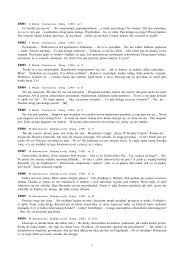
5000 uniform variates
a = 1229, b = 1, M = 2048, s0 = 1
Computational Finance – p. 4

Are the numbers Ui obtained with the congruential linear
generator uniformly distributed? It seems so, as the histogram
is quite flat.
Does this really means, that the numbers Ui are good uniform
deviates?
There is a question whether they are independent. To study
this property we consider vectors built of Ui’s:
(Ui,Ui+1,...,Ui+m−1) ∈ [0, 1] m
and analyze them with respect to distribution.
If Ui’s are good uniform deviates, above random vectors are
uniformly distributed over [0, 1] m .
It should be stressed that it is very difficult to assess random
number generators!
Computational Finance – p. 5

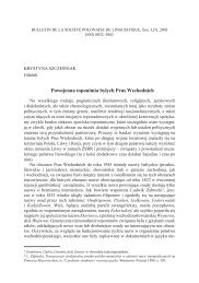
The plot of pairs (Ui,Ui+1) for the linear congruential generator
with a = 1229, b = 1, M = 2048.
Computational Finance – p. 6

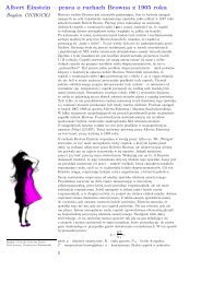
Good congruential generator with a = 1597, b = 51749 and
M = 244944
Computational Finance – p. 7

Deceptively good congruential generator with a = 2 16 + 3,
b = 0, M = 2 31
Computational Finance – p. 8

Apparently not so good congruential generator with
a = 2 16 + 3, b = 0, M = 2 31
Computational Finance – p. 9

In general Marsaglia showed that the m-tuples
(Ui,...,Ui+m−1) generated with linear congruential generators
lie on relatively low number of hyperplanes in R m .
This is a major disadvantage of linear congruential generators.
An alternative way to generate uniform deviates is by using
Fibonacci generators.
Computational Finance – p. 10

Fibonacci generators
The original Fibonacci recursion motivates the following
general approach to generate pseudo-random numbers
si = si−n op si−k.
Here 0 < k < n are the lags and op can be one of the following
operators:
+ addition mod M,
− subtraction mod M,
∗ multiplication mod M.
To initialize (seed) these generators we have to use another
generator to supply first n numbers s0, s1, . . . , sn−1. In
addition, in subtraction generators we have to control that if
si < 0 for some i the result has to be shifted si := si + M.
Computational Finance – p. 11

What are ”good generators”?
Good generators are those generators that pass a large
number of statistical tests, see, e.g.,
P. L’Ecuyer and R. Simard – TestU01: A C Library for Empirical Testing of Random Number
Generators, ACM Transactions on Mathematical Software, Vol. 33, article 22, 2007
TestU01 is a software library, implemented in C, and offering a
collection of utilities for the empirical statistical testing of
uniform random number generators.
These tests are freely accessible on the web page
http://www.iro.umontreal.ca/ simardr/testu01/tu01.html
Computational Finance – p. 12

”Minimal Standard” generators
W. H. Press, S. A. Teukolsky, W. T. Vetterling, B. P. Flannery – Numerical Recipes in C
offers a number of portable random number generators, which
passed all new theoretical tests, and have been used
successfully.
The simplest of these generators, called ran0, is a standard
congruential generator
si+1 = asi mod M,
with a = 7 5 = 16807 and M = 2 31 − 1, is a basis for more
advanced generators ran1 and ran2. There are also better
generators like ran3 and ran4.
Of these generators only ran3 possesses sufficiently good
properties to be used in financial calculations.
It can be difficult or impossible to implement these generators
directly in a high-level language, since usually integer
arithmetics is limited to 32 bits. Computational Finance – p. 13

To avoid this difficulty Schrage proposed an algorithm for
multiplying two 32-bit integers modulo a 32-bit constant,
without using any intermediates larger than 32 bits. Schrage’s
algorithm is based on an approximate factorization of M
M = aq + r, i.e. q = [M/a], r = M mod a.
If r < q , and 0 < z < M − 1, it can be shown that both
a(z mod q) and r[z/q] lie in the range [0,M − 1]. Then
az mod M =
�
a(z mod q) − r[z/q], if it is ≥ 0,
a(z mod q) − r[z/q] + M, otherwise.
For ran0 Schrage’s algorithm is uses with the values
q = 127773 and r = 2836.
Computational Finance – p. 14

The Mersenne Twister
The Mersenne Twister of Matsumoto and Nishimura which
appeared in late 90-ties is now mostly used in financial
simulations.
It has a period of 2 19937 − 1 and the correlation effect is not
observed for this generator up to dimension 625.
Mersenne Twister is now implemented in most commercial
packages. In particular, it is a standard generator in Matlab,
Octave, R-project, S-plus.
Computational Finance – p. 15

Generation of uniform
pseudo-random numbers
The generator of pseudo-random numbers with uniform
distribution on interval [0, 1] in Octave can be called by one of
the commands:
rand (x)
rand (n, m)
rand ("state", v)
The version rand (x) returns x-dimensional square matrix
of uniformly distributed pseudo-random numbers.
For two scalar arguments, rand takes them to be the number
of rows and columns.
Computational Finance – p. 16

The state of the random number generator can be queried
using the form
v = rand ("state")
This returns a column vector v of length 625. Later, the
random number generator can be restored to the state v using
the form
rand ("state", v)
The state vector may be also initialized from an arbitrary
vector of length ≤ 625 for v. By default, the generator is
initialized from /dev/urandom if it is available, otherwise from
CPU time, wall clock time and the current fraction of a second.
Computational Finance – p. 17

and includes a second random number generator, which
was the previous generator used in Octave. If in some
circumstances it is desirable to use the old generator, the
keyword "seed" is used to specify that the old generator
should be used.
The generator in such situation has to be initialized as in
rand ("seed", v)
which sets the seed of the generator to v.
It should be noted that most random number generators
coming with C++ work fine, they are usually congruential
generators, so you should be aware of their limitations.
Computational Finance – p. 18

Generation of non-uniformly
distributed random deviates
Idea 1: Discrete distributions
Idea 2: Inversion of the distribution function
Idea 3: Transformation of random variables
Computational Finance – p. 19

Idea 1: Discrete distributions
Coin toss distribution: P(X = 1) = 0.5, P(X = 0) = 0.5
(1) Generate U ∼ U(0, 1)
(2) If U ≤ 0.5 then Z = 1, otherwise Z = 0
Z has a coin toss distribution.
Discrete distribution: P(X = ai) = pi, i = 1, 2,... ,n
(1) Compute ck = � k
i=1 pi
(2) Generate U ∼ U(0, 1)
(3) Find smallest k such that U ≤ ck. Put Z = ak
Z has a given discrete distribution.
Computational Finance – p. 20

Idea 2: Inversion of the distribution function
Proposition. Let U ∼ U(0, 1) and F be a continuous and
strictly increasing cumulative distribution function. Then
F −1 (U) is a sample of F .
Theoretically this approach seems to be fine. The only thing
we really need to do is to generate uniformly distributed
random numbers.
Works well for: exponential distribution, uniform distribution on
various intervals, Cauchy distribution.
Computational Finance – p. 21

Beasley-Springer-Moro algorithm for normal variate uses
inversion of the distribution function with high accuracy
(3 × 10 −9 ).
In interval 0.5 ≤ y ≤ 0.92 the algorithm uses the formula
F −1 (y) ≈
and for y ≥ 0.92 the formula
F −1 (y) ≈
� 3
n=0 an(y − 0.5) 2n+1
1 + � 3
n=0 bn(y − 0.5) 2n,
8�
n=0
cn
�
log � − log(1 − y) �� n
.
Computational Finance – p. 22

Idea 3: Transformation of random variables
Proposition. Let X be a random variable with density function
f on the set A = {x ∈ R n |f(x) > 0}. Assume that the
transformation h : A → B = h(A) is invertible and that the
inverse h −1 is continuously differentiable. Then Y = h(X) has
the density
for all y ∈ B.
y ↦→ f(h −1 (y)) ·
�
�
�
�det �
dh−1 dy (y)
��
���
,
Computational Finance – p. 23

Multidimensional normal distribution N(µ, Σ) on R p has a
density
f(x) =
1
(2π) p/2
1
�
exp
(det Σ) 1/2
− 1
2 (x − µ)TΣ −1 �
(x − µ) .
Here µ is a p-dimensional vector of expected values, and Σ is
a p × p-dimensional covariance matrix.
Computational Finance – p. 24

If X ∼ N(µ, Σ), then
X = (X1,X2,...,Xp),
µ = EX = (EX1,...,EXp)
Σ = (Σij)i,j=1,...,p is a square matrix, where
Σij = Σji,
Σii = var(Xi)
Σij = cov(Xi,Xj) = E[(Xi − µi)(Xj − µj)]
Computational Finance – p. 25

We are going to apply this result for the case where A = [0, 1] 2
and f(x) = 1 for all x ∈ A (i.e. we start with a two-dimensional
uniformly distributed random variable) and choose the
transformation
x ↦→ h(x) =
�√−2 �
ln x1 cos(2πx2),
√
−2 ln x1 sin(2πx2).
The inverse of this transformation is given by
y ↦→ h −1 �
exp(−�y�
(y) =
2 �
/2),
arctan(y2/y1)/2π.
Computational Finance – p. 26

We compute the determinant of the derivative at y = h(x) as
follows:
det
�
dh−1 dy (y)
�
= − 1
2π exp
�
− 1
2 (y2 1 + y 2 �
2)
Therefore, the density function of Y = h(X), where
X ∼ U([0, 1] 2 ) equals
f � h −1 (y) � ·
� �
� dh−1 � det
dy (y)
��
��
= 1 · 1
2π exp
�
− 1
2 (y2 1 + y 2 �
2) .
This is obviously the density function of the two-dimensional
standard normal distribution.
We therefore obtain that h(X) is 2-dimensional standard
normally distributed, whenever X is uniformly distributed on
[0, 1] 2 .
Computational Finance – p. 27

Creates Z ∼ N(0, 1):
Box-Muller algorithm
1. Generate U1 ∼ U[0, 1] and U2 ∼ U[0, 1],
2. θ = 2πU2, ρ = √ −2 log U1,
3. Z1 := ρcos θ is a normal variate (as well as Z2 := ρsin θ).
Computational Finance – p. 28

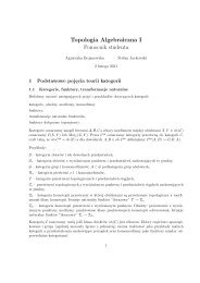
Box-Muller with congruential generator
Computational Finance – p. 29

Naeve effect
In 1973, H. R. Naeve discovered an undesirable interaction
between simple multiplicative congruential pseudo-random
number generators and the Box-Muller algorithm. The pairs of
points generated by the Box-Muller method fall into a small
range (rectangle) around zero. The Naeve effect disappears
for the polar method.
Unfortunately, number theorists suspect that effects similar to
the Naeve effect may occur for other pseudo-random
generators.
In summary, since there are highly accurate algorithms for the
inverse cumulative normal probability function, use those
rather than the Box-Muller algorithm.
Computational Finance – p. 30

Marsaglia algorithm
The Box-Muller algorithm has been improved by Marsaglia in
a way that the use of trigonometric functions can be avoided.
It is important, since computation of trigonometric functions is
very time-consuming.
Algorithm: polar method (creates Z ∼ N(0, 1)):
1. repeat generate U1,U2 ∼ U[0, 1];
V1 = 2U1 − 1, V2 = 2U2 − 1;
until W := V 2
1 + V 2
2 < 1.
�
2. Z1 := V1 −2 ln(W)/W
�
Z2 := V2 −2 ln(W)/W
are both normal variates.
Computational Finance – p. 31

Generation of N(µ,σ 2 ) distributed pseudo-random
variables
(1) Compute Z ∼ N(0, 1)
(2) Z1 = µ + σZ
Z1 is a pseudo-random number from a normal distribution
N(µ,σ 2 ).
Computational Finance – p. 32

How to generate a sample from a multidimensional normal
distribution?
Theorem. Let Z be a vector of p independent random
variables each with a standard normal distribution N(0, 1).
There exists a matrix A such that
µ + AZ ∼ N(µ, Σ).
Our aim is to find such a matrix A. We know how to generate
a sequence of independent normally distributed random
variables. Using matrix A we can transform it into a sequence
of multidimensional normal variates.
Computational Finance – p. 33

The covariance matrix Σ is positive definite. One can show
that there is exactly one lower-triangular matrix A with positive
diagonal elements, s.t.
Σ = A · A T ,
where A T denotes a transpose of a matrix A.
This decomposition is called the Cholesky decomposition.
There are numerical methods how to compute the Cholesky
decomposition of a positive definite matrix, but we don’t
discuss this here.
Computational Finance – p. 34

Algorithm for generation of N(µ, Σ) distributed pseudo-random
variables.
1. Calculate the Cholesky decomposition AA T = Σ.
2. Calculate Z ∼ N(0,I) componentwise by Zi ∼ N(0, 1),
i = 1,...,n, for instance with Marsaglia polar algorithm.
3. µ + AZ has the desired distribution ∼ N(µ, Σ).
Computational Finance – p. 35

Constant correlation Brownian motion
We call a process W(t) = (W1(t),...,Wd(t)) a standard
d-dimensional Brownian motion when the coordinate
processes Wi(t) are standard one-dimensional Brownian
motions with Wi and Wj independent for i �= j.
Let µ be a vector in R d and Σ an d × d positive definite matrix.
We call a process X a Brownian motion with drift µ and
covariance Σ if X has continuous sample paths and
independent increments with
X(t + s) − X(s) ∼ N(tµ,tΣ).
Process X is called a constant correlation Brownian motion
(which means that Σ is constant).
Computational Finance – p. 36

Simulation
For Monte Carlo simulations with correlated Brownian motion
we have to know how to generate samples from N(δtµ,δtΣ).
Since δt is a known constant we can reduce the problem to
generating samples from distribution N(µ, Σ).
Methods of sample generation:
Cholesky decomposition (discussed earlier),
PCA construction.
Computational Finance – p. 37

Cholesky decomposition
Algorithm for generation of N(µ, Σ) distributed pseudo-random
variables:
1. Calculate the Cholesky decomposition AA T = Σ.
2. Calculate Z ∼ N(0,I) componentwise by Zi ∼ N(0, 1),
i = 1,...,n.
3. µ + AZ has the desired distribution ∼ N(µ, Σ).
Computational Finance – p. 38

PCA construction
Principal Component Analysis (PCA) is the method of
analyzing spectrum of the covariance matrix.
Since Σ is symmetric positive definite matrix, it has d positive
eigenvalues and d eigenvectors which span the space R d . In
addition the following formula holds
Σ = ΓΛΓ T ,
where Γ is the matrix of d eigenvectors of Σ and Λ is the
diagonal matrix of eigenvalues of Σ.
Computational Finance – p. 39

Theorem. Let Z be a vector of d independent random
variables each with a standard normal distribution N(0, 1).
Then
µ + ΓΛ 1/2 Z ∼ N(µ, Σ),
where Σ = ΓΛΓ T is the spectral decomposition of matrix Σ.
Let us observe that due to positivity of eigenvalues Λ 1/2 is well
defined.
Computational Finance – p. 40

In general Cholesky decomposition and PCA construction do
not give the same results.
Indeed
and
holds. But in general
Σ = AA T = ΓΛΓ T = ΓΛ 1/2 Λ 1/2 Γ T
Σ(A T ) −1 = A = ΓΛ 1/2 Λ 1/2 Γ T (A T ) −1
Λ 1/2 Γ T (A T ) −1 �= I,
where I is the identity matrix. Hence
AZ �= ΓΛ 1/2 Z
even though both sides generate correlated deviates.
Computational Finance – p. 41

Computer implementation
In a Cholesky factorization matrix A is lower triangular. It
makes calculations of AZ particularly convenient because it
reduces the calculations complexity by a factor of 2 compared
to the multiplication of Z by a full matrix ΓΛ 1/2 . In addition
error propagates much slower in Cholesky factorization.
Cholesky factorization is more suitable to numerical
calculations than PCA.
Why use PCA?
The eigenvalues and eigenvectors of a covariance matrix have
statistical interpretation that is some times useful. Examples
of such a usefulness are in some variance reduction methods.
Computational Finance – p. 42