Modelling Bridge Piers and Afflux in TUFLOW
Modelling Bridge Piers and Afflux in TUFLOW
Modelling Bridge Piers and Afflux in TUFLOW

Create successful ePaper yourself
Turn your PDF publications into a flip-book with our unique Google optimized e-Paper software.
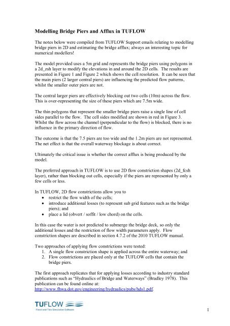
<strong>Modell<strong>in</strong>g</strong> <strong>Bridge</strong> <strong>Piers</strong> <strong>and</strong> <strong>Afflux</strong> <strong>in</strong> <strong>TUFLOW</strong><br />
The notes below were compiled from <strong>TUFLOW</strong> Support emails relat<strong>in</strong>g to modell<strong>in</strong>g<br />
bridge piers <strong>in</strong> 2D <strong>and</strong> estimat<strong>in</strong>g the bridge afflux; always an <strong>in</strong>terest<strong>in</strong>g topic for<br />
numerical modellers!<br />
The model provided uses a 5m grid <strong>and</strong> represents the bridge piers us<strong>in</strong>g polygons <strong>in</strong><br />
a 2d_zsh layer to modify the elevations <strong>in</strong> <strong>and</strong> around the 2D cells. The results are<br />
presented <strong>in</strong> Figure 1 <strong>and</strong> Figure 2 which shows the cell resolution. It can be seen that<br />
the ma<strong>in</strong> piers (2 larger central piers) are <strong>in</strong>fluenc<strong>in</strong>g the predicted flow patterns,<br />
whilst the smaller outer piers are not.<br />
The central larger piers are effectively block<strong>in</strong>g out two cells (10m) across the flow.<br />
This is over-represent<strong>in</strong>g the size of these piers which are 7.5m wide.<br />
The th<strong>in</strong> polygons that represent the smaller bridge piers raise a s<strong>in</strong>gle l<strong>in</strong>e of cell<br />
sides parallel to the flow. The cell sides modified are shown <strong>in</strong> red <strong>in</strong> Figure 3.<br />
Whilst the flow across the channel (perpendicular to the flow) is blocked, there is no<br />
<strong>in</strong>fluence <strong>in</strong> the primary direction of flow.<br />
The outcome is that the 7.5 piers are too wide <strong>and</strong> the 1.2m piers are not represented.<br />
The net effect is that the overall waterway blockage is about correct.<br />
Ultimately the critical issue is whether the correct afflux is be<strong>in</strong>g produced by the<br />
model.<br />
The preferred approach <strong>in</strong> <strong>TUFLOW</strong> is to use 2D flow constriction shapes (2d_fcsh<br />
layer), rather than block<strong>in</strong>g out cells, especially if the piers are represented by only a<br />
few cells or less.<br />
In <strong>TUFLOW</strong>, 2D flow constrictions allow you to<br />
restrict the flow width of the cells;<br />
<strong>in</strong>troduce additional losses (to represent sub grid features such as the bridge<br />
piers); <strong>and</strong><br />
place a lid (obvert / soffit / low chord) on the cells.<br />
In this case the water is not predicted to submerge the bridge deck, so only the<br />
additional losses <strong>and</strong> the restriction of flow width parameters apply. Flow<br />
constriction shapes are described <strong>in</strong> section 4.7.2 of the 2010 <strong>TUFLOW</strong> manual.<br />
Two approaches of apply<strong>in</strong>g flow constrictions were tested:<br />
1. A s<strong>in</strong>gle flow constriction shape is applied across the entire waterway; <strong>and</strong><br />
2. Flow constrictions are placed only at the <strong>TUFLOW</strong> cells that conta<strong>in</strong> the<br />
bridge piers.<br />
The first approach replicates that for apply<strong>in</strong>g losses accord<strong>in</strong>g to <strong>in</strong>dustry st<strong>and</strong>ard<br />
publications such as “Hydraulics of <strong>Bridge</strong> <strong>and</strong> Waterways” (Bradley 1978). This<br />
publication can be found onl<strong>in</strong>e at:<br />
http://www.fhwa.dot.gov/eng<strong>in</strong>eer<strong>in</strong>g/hydraulics/pubs/hds1.pdf.<br />
1
The second approach is an adaptation of the same logic but allows the modeller to<br />
apply the parameters only to the 2D cells that conta<strong>in</strong> the bridge piers. This has the<br />
advantage of produc<strong>in</strong>g more realistic flow patterns, <strong>and</strong> represent<strong>in</strong>g each bridge pier<br />
<strong>in</strong>dividually rather than lumped together.<br />
Hydraulics of <strong>Bridge</strong> <strong>and</strong> Waterways estimates the additional losses based on the pier<br />
shape <strong>and</strong> fraction of the waterway blocked. A backwater coefficient is determ<strong>in</strong>ed<br />
us<strong>in</strong>g the charts provided, <strong>and</strong> is applied <strong>in</strong> <strong>TUFLOW</strong> as an energy loss based on the<br />
velocity head.<br />
2<br />
V<br />
h <br />
a 2g<br />
Where <br />
a<br />
is the calculated coefficient, based on the figures/charts <strong>in</strong> Bradley (1978).<br />
This figure is reproduced here <strong>in</strong> Figure 4.<br />
For calculat<strong>in</strong>g the J value (fraction of the area blocked by piers), the entire bridge<br />
open<strong>in</strong>g is determ<strong>in</strong>ed for the first approach (one form loss value for the entire bridge,<br />
see Figure 5), <strong>and</strong> for each <strong>in</strong>dividual span for the second approach as discussed<br />
below (example pier shown <strong>in</strong> Figure 6).<br />
Approach 1:<br />
The entire bridge the length is approximately 270m <strong>and</strong> there are 19.8m of bridge<br />
piers (4 by 1.2m piers <strong>and</strong> 2 by 7.5m piers). This equates to a Blockage fraction (J<br />
value) of 0.073. Us<strong>in</strong>g the Hydraulics of <strong>Bridge</strong> <strong>and</strong> Waterways chart (Figure 4) <strong>and</strong><br />
assum<strong>in</strong>g a s<strong>in</strong>gle rounded pier shape a form loss coefficient (∆Kp) of 0.14 is<br />
determ<strong>in</strong>ed. This method is presented visually <strong>in</strong> Figure 5 <strong>and</strong> Figure 7.<br />
Approach 2:<br />
The calculation is repeated for each <strong>in</strong>dividual pier by assess<strong>in</strong>g the flow area blocked<br />
on a span by span approach, <strong>in</strong> a similar method to a parallel channel analysis. For<br />
each pier, the flow width from mid pier to mid pier is calculated, <strong>and</strong> the pier width is<br />
used to calculate a J value for each pier. This is shown visually <strong>in</strong> Figure 6.<br />
Us<strong>in</strong>g the same method as above a pier coefficient (∆Kp) can be determ<strong>in</strong>ed for each<br />
pier. As the flow constriction is only applied to the <strong>TUFLOW</strong> cells where the bridge<br />
piers are, this loss (∆Kp) is factored, based on the number of cells <strong>in</strong> the span <strong>and</strong> the<br />
number of bridge pier cells. For example, if the bridge span is 50m (as <strong>in</strong> Figure 6),<br />
this is 10 <strong>TUFLOW</strong> cells, however the 7.5m pier is only modelled with 2 <strong>TUFLOW</strong><br />
cells. In this case the calculated ∆Kp is multiplied by 5 (ie. 10/2).<br />
The additional (∆Kp) form loss values <strong>and</strong> blockage width to the <strong>TUFLOW</strong> cells are<br />
applied us<strong>in</strong>g the 2d_fcsh layer attributes. For this second approach care has been<br />
taken to apply this to the correct number of <strong>TUFLOW</strong> cells.<br />
Analysis:<br />
For both of the approaches described above the flow constrictions have been setup<br />
with <strong>and</strong> without additional blockages be<strong>in</strong>g applied to the <strong>TUFLOW</strong> cells. The logic<br />
2
eh<strong>in</strong>d this is that the Hydraulics of <strong>Bridge</strong> Waterways accounts for the blockage <strong>and</strong><br />
so <strong>in</strong>clud<strong>in</strong>g the blockage on the <strong>TUFLOW</strong> cells may over-represent the losses.<br />
A comparison of the different approaches is presented below. The five approaches<br />
analysed are:<br />
Table 1 <strong>Bridge</strong> Pier <strong>Modell<strong>in</strong>g</strong> Approaches<br />
Scenario<br />
No <strong>Bridge</strong><br />
Scen1<br />
Scen2<br />
Scen3<br />
Scen4<br />
Scen5<br />
Description<br />
No bridge piers <strong>in</strong>cluded<br />
<strong>Bridge</strong> piers <strong>in</strong>cluded by block<strong>in</strong>g out the cells (rais<strong>in</strong>g elevations).<br />
This is the method used <strong>in</strong> the model provided to <strong>TUFLOW</strong> Support.<br />
S<strong>in</strong>gle form loss coefficient applied across entire waterway, ie. form<br />
loss applies to all cells across river. Form Loss Coefficient (FLC) =<br />
0.14<br />
As for Scen2 but percentage blockage also applied, ie. loss <strong>and</strong><br />
blockage applies to all cells across the river. Form Loss Coefficient =<br />
0.14, blockage = 7.3%<br />
Form loss calculated per bridge span <strong>and</strong> applied only at pier cells.<br />
No blockage applied. The FLC values adopted for the smaller piers<br />
were 0.07 (1.2m pier <strong>in</strong> 30m waterway), this was factored to 0.42 to<br />
apply only at the pier cells. For the larger piers the unfactored FLC<br />
was 0.32 which was factored to 1.60, to apply only at the pier cells..<br />
As for Scen4 but blockage also applied. For example at a 1.2m pier<br />
with a 5m cell, a 24% blockage is applied at pier cells.<br />
The velocity magnitudes <strong>and</strong> directions for the methods above are presented <strong>in</strong> Figure<br />
8 through to Figure 13.<br />
A water level profile was extracted <strong>in</strong> the vic<strong>in</strong>ity of the bridge for each scenario; the<br />
location of the profile extraction is presented <strong>in</strong> Figure 14. The water level profiles are<br />
shown below <strong>in</strong> Figure 15, for the 20 Year event.<br />
Predicted velocities <strong>in</strong> the vic<strong>in</strong>ity of the bridge are generally less than 1 metre per<br />
second. Average velocities through the bridge section range from 0.54 to 0.61 m/s<br />
(depend<strong>in</strong>g on the method of modell<strong>in</strong>g the bridge). These are detailed <strong>in</strong> the table<br />
below for the 5 scenarios. The average velocities <strong>in</strong> the table below are calculated<br />
from the flow through the bridge divided by the flow area through the bridge.<br />
3
Table 2 Average Velocities Through <strong>Bridge</strong> Structure<br />
Scenario Average Velocity (m/s)<br />
No <strong>Bridge</strong> 0.54<br />
Scen1 0.61<br />
Scen2 0.54<br />
Scen3 0.58<br />
Scen4 0.54<br />
Scen5 0.60<br />
These low velocities produce the small affluxes shown <strong>in</strong> Figure 15. An afflux<br />
calculation for the piers based on the Hydraulics of <strong>Bridge</strong> Waterways method was<br />
carried out as an <strong>in</strong>dependent check. The values used were the predicted average<br />
velocity <strong>and</strong> the calculated <strong>in</strong>cremental backwater coefficient for piers (∆Kp) of 0.14.<br />
The afflux calculated is 2.6mm (see Table 3).<br />
Table 3 <strong>Afflux</strong> Due to <strong>Bridge</strong> Pier Desktop Calculations<br />
Parameter Description<br />
0.61 Predicted Average Velocity (m/s)<br />
0.019 Dynamic Head (v2/2g)<br />
0.00263 <strong>Afflux</strong> (m)<br />
2.63 <strong>Afflux</strong> (mm)<br />
<strong>Afflux</strong>es were calculated across the bridge by subtract<strong>in</strong>g the water level at cha<strong>in</strong>age<br />
390m from 490m. For each of the methods of modell<strong>in</strong>g the bridges, the total afflux is<br />
calculated as well as the <strong>in</strong>crease <strong>in</strong> afflux compared to the scenario without the<br />
bridge <strong>in</strong> the model. The afflux has been calculated as the <strong>in</strong>crease <strong>in</strong> water level<br />
upstream due to the bridge.<br />
The approaches that block out the <strong>in</strong>dividual 2D cells (Scen1 <strong>and</strong> Scen5, 4.4 <strong>and</strong><br />
4.9mm) overestimate the afflux compared with the Hydraulics of <strong>Bridge</strong> Waterways<br />
method (2.6mm).<br />
Scenario<br />
Table 4 Modelled <strong>Afflux</strong>es 20 Year Event<br />
Total Head<br />
Drop (mm)<br />
<strong>Afflux</strong><br />
(Compared to No <strong>Bridge</strong>) (mm)<br />
No <strong>Bridge</strong> 3.3 -<br />
Scen1 7.7 4.4<br />
Scen2 5.5 2.2<br />
Scen3 5.9 2.5<br />
Scen4 6.0 2.6<br />
Scen5 8.2 4.9<br />
HBW --- 2.6<br />
4
In order to test the losses under higher velocities, the model was run with a multiplier<br />
of five (5) on the flows whilst the downstream tail water was left unchanged. The<br />
average velocities for this case are presented below <strong>in</strong> Table 5, with the highest<br />
velocities be<strong>in</strong>g around 2.5m/s for this event.<br />
The velocity magnitude <strong>and</strong> directions for the 5 x 20yr <strong>in</strong>flow event are presented <strong>in</strong><br />
Figure 16 through to Figure 21.<br />
Table 5 Average Velocities Through the <strong>Bridge</strong> Structure; 5 x 20yr Inflows<br />
Scenario Average Velocity (m/s)<br />
No <strong>Bridge</strong> 1.87<br />
Scen1 2.04<br />
Scen2 1.87<br />
Scen3 2.01<br />
Scen4 1.87<br />
Scen5 2.08<br />
The profiles for this case are presented below <strong>in</strong> Figure 22. The afflux calculation<br />
us<strong>in</strong>g Hydraulic of <strong>Bridge</strong> Waterways is presented <strong>in</strong> Table 6. This afflux calculation<br />
depends on which modelled velocity from the table above is used, the afflux ranges<br />
from 25mm to 31mm.<br />
Table 6 <strong>Afflux</strong> from Desktop Calculations; 5 x 20yr Inflows<br />
Lower Range Upper Range Description<br />
1.87 2.08 Predicted Average Velocity (m/s)<br />
0.178 0.220 Dynamic Head (v 2 /2g)<br />
0.0250 0.0309 <strong>Afflux</strong> (m)<br />
25.0 30.9 <strong>Afflux</strong> (mm)<br />
The modelled affluxes across the bridge structure for the five scenarios are presented<br />
<strong>in</strong> Table 7.<br />
Based on the results Scen2 (28mm) gives the closest results to the Hydraulics of<br />
<strong>Bridge</strong> <strong>and</strong> Waterways calculation of 25mm to 31mm. The case with the bridge<br />
modelled by block<strong>in</strong>g out the cells (central piers only), produces the highest afflux<br />
(51mm) <strong>and</strong> overestimates the losses, compared to the Hydraulic of <strong>Bridge</strong><br />
Waterways calculation.<br />
5
Scenario<br />
Table 7 <strong>Afflux</strong>es Across <strong>Bridge</strong>; 5 x 20yr Inflows<br />
Total Head<br />
Drop (mm)<br />
<strong>Afflux</strong><br />
(Compared to No <strong>Bridge</strong>) (mm)<br />
No <strong>Bridge</strong> 28 -<br />
Scen1 79 51<br />
Scen2 56 28<br />
Scen3 61 33<br />
Scen4 61 33<br />
Scen5 68 40<br />
HBW --- 25 to 31<br />
Conclusion:<br />
Whilst the approaches that remove or block the cells at the piers produce what would<br />
appear as more realistic flow patterns, care needs to be taken to ensure that the<br />
affluxes predicted are representative. This model <strong>and</strong> other modell<strong>in</strong>g carried out<br />
us<strong>in</strong>g a variety of 2D software (fixed grid <strong>and</strong> flexible mesh) tends to show that<br />
block<strong>in</strong>g out cells/elements for bridge piers will overestimate the afflux compared to<br />
the Hydraulics of <strong>Bridge</strong> Waterways approach.<br />
There are a number of methods <strong>in</strong> <strong>TUFLOW</strong> for modell<strong>in</strong>g of bridges that allow the<br />
modeller to apply parameters from publications such as the Hydraulics of <strong>Bridge</strong><br />
Waterways. As with any numerical model outputs, it is essential that these models are<br />
used with<strong>in</strong> their capabilities to ensure the results produced are truly representative of<br />
the bridge afflux.<br />
In this document we have not explored <strong>TUFLOW</strong>’s capabilities for modell<strong>in</strong>g bridges<br />
<strong>in</strong> 2D once the bridge deck has become submerged. <strong>TUFLOW</strong> is able to model this<br />
situation, but like all modell<strong>in</strong>g, cross-check<strong>in</strong>g through benchmark<strong>in</strong>g to established<br />
publications <strong>and</strong> theory is an important part of the modell<strong>in</strong>g process.<br />
For complex or poorly understood obstructions to flow, Computational Fluid<br />
Dynamics (CFD) may be required as another means of establish<strong>in</strong>g the losses that can<br />
then be applied to 2D solvers such as <strong>TUFLOW</strong>.<br />
Figures:<br />
6
Figure 1 Velocity Magnitude <strong>and</strong> Direction; <strong>Piers</strong> Modelled by Modify<strong>in</strong>g the Zpts<br />
7
Figure 2 <strong>TUFLOW</strong> Grid Resolution<br />
Figure 3 <strong>TUFLOW</strong> Cells <strong>and</strong> Pier Locations; 5m model<br />
8
Figure 4 Incremental Backwater Coefficient for <strong>Piers</strong> (Hydraulics of <strong>Bridge</strong> <strong>and</strong> Waterways, 1978)<br />
9
Figure 5 Blockage Calculation for Entire <strong>Bridge</strong> (Cell Size Independent)<br />
Figure 6 Blockage Calculation at Example Span<br />
10
Figure 7 Formloss Coefficient for Entire <strong>Bridge</strong><br />
Figure 8 Velocity Magnitude <strong>and</strong> Direction, 20yr Inflow; No <strong>Bridge</strong><br />
11
Figure 9 Velocity Magnitude <strong>and</strong> Direction, 20yr Inflow; Scen1<br />
Figure 10 Velocity Magnitude <strong>and</strong> Direction, 20yr Inflow; Scen2<br />
12
Figure 11 Velocity Magnitude <strong>and</strong> Direction, 20yr Inflow; Scen3<br />
Figure 12 Velocity Magnitude <strong>and</strong> Direction, 20yr Inflow; Scen4<br />
13
Figure 13 Velocity Magnitude <strong>and</strong> Direction, 20yr Inflow; Scen5<br />
Figure 14 Profile Extraction Location<br />
14
Figure 15 Water Surface Profiles; <strong>Bridge</strong> <strong>Modell<strong>in</strong>g</strong> Methods<br />
Figure 16 Velocity Magnitude <strong>and</strong> Direction, 5 x 20yr Inflow; No <strong>Bridge</strong><br />
15
Figure 17 Velocity Magnitude <strong>and</strong> Direction, 5 x 20yr Inflow; Scen1<br />
Figure 18 Velocity Magnitude <strong>and</strong> Direction, 5 x 20yr Inflow; Scen2<br />
16
Figure 19 Velocity Magnitude <strong>and</strong> Direction, 5 x 20yr Inflow; Scen3<br />
Figure 20 Velocity Magnitude <strong>and</strong> Direction, 5 x 20yr Inflow; Scen4<br />
17
Figure 21 Velocity Magnitude <strong>and</strong> Direction, 5 x 20yr Inflow; Scen5<br />
Figure 22 Water Surface Profiles, 5 x 20yr Inflows<br />
18