2D Modelling Approaches for Buildings and Fences - TUFLOW

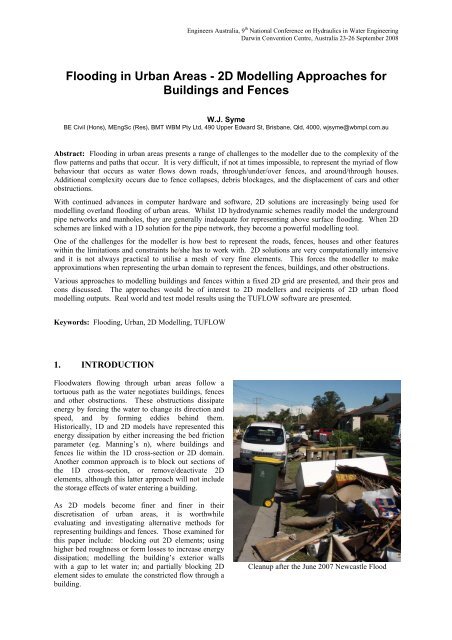
Engineers Australia, 9 th National Conference on Hydraulics in Water EngineeringDarwin Convention Centre, Australia 23-26 September 2008Flooding in Urban Areas - 2D Modelling Approaches forBuildings and FencesW.J. SymeBE Civil (Hons), MEngSc (Res), BMT WBM Pty Ltd, 490 Upper Edward St, Brisbane, Qld, 4000, wjsyme@wbmpl.com.auAbstract: Flooding in urban areas presents a range of challenges to the modeller due to the complexity of theflow patterns and paths that occur. It is very difficult, if not at times impossible, to represent the myriad of flowbehaviour that occurs as water flows down roads, through/under/over fences, and around/through houses.Additional complexity occurs due to fence collapses, debris blockages, and the displacement of cars and otherobstructions.With continued advances in computer hardware and software, 2D solutions are increasingly being used formodelling overland flooding of urban areas. Whilst 1D hydrodynamic schemes readily model the undergroundpipe networks and manholes, they are generally inadequate for representing above surface flooding. When 2Dschemes are linked with a 1D solution for the pipe network, they become a powerful modelling tool.One of the challenges for the modeller is how best to represent the roads, fences, houses and other featureswithin the limitations and constraints he/she has to work with. 2D solutions are very computationally intensiveand it is not always practical to utilise a mesh of very fine elements. This forces the modeller to makeapproximations when representing the urban domain to represent the fences, buildings, and other obstructions.Various approaches to modelling buildings and fences within a fixed 2D grid are presented, and their pros andcons discussed. The approaches would be of interest to 2D modellers and recipients of 2D urban floodmodelling outputs. Real world and test model results using the TUFLOW software are presented.Keywords: Flooding, Urban, 2D Modelling, TUFLOW1. INTRODUCTIONFloodwaters flowing through urban areas follow atortuous path as the water negotiates buildings, fencesand other obstructions. These obstructions dissipateenergy by forcing the water to change its direction andspeed, and by forming eddies behind them.Historically, 1D and 2D models have represented thisenergy dissipation by either increasing the bed frictionparameter (eg. Manning’s n), where buildings andfences lie within the 1D cross-section or 2D domain.Another common approach is to block out sections ofthe 1D cross-section, or remove/deactivate 2Delements, although this latter approach will not includethe storage effects of water entering a building.As 2D models become finer and finer in theirdiscretisation of urban areas, it is worthwhileevaluating and investigating alternative methods forrepresenting buildings and fences. Those examined forthis paper include: blocking out 2D elements; usinghigher bed roughness or form losses to increase energydissipation; modelling the building’s exterior wallswith a gap to let water in; and partially blocking 2Delement sides to emulate the constricted flow through abuilding.Cleanup after the June 2007 Newcastle Flood

Engineers Australia, 9 th National Conference on Hydraulics in Water EngineeringDarwin Convention Centre, Australia 23-26 September 20082. REPRESENTATION OFBUILDINGS2.1 Increased RoughnessIncreasing the bed resistance parameter is acommonly used method for representing theincreased energy dissipation of water flowingthrough and around buildings. It is oftenfavoured over blocking out the building as itincludes the storage effects of the buildingbeing inundated. The parameter may also bevaried. For example, a lower Manning’s nFigure 2.1 – Example of Using Higher Roughness for Housesvalue can be used for houses and gardensand Gardens (Throsby Creek Flood Study courtesy Newcastle CC)compared with a higher value for commercialproperties on the basis that residential areas are less “dense” thancommercial areas. Figure 2.1 shows TUFLOW output for a20m Cellsmodel where higher roughness was used for urban areas asBreachillustrated by the higher velocities on the roads and lowervelocities through the houses and gardens.Varying the Manning’s n value also works well when theresolution of the 2D elements is coarse. For example, a fixedgrid model using 10m square cells will struggle to adequatelyrepresent the flow between buildings if the buildings have beenblocked out (as illustrated by the images in Figure 2.2), whereasvarying the Manning’s n value is somewhat less sensitive to thiseffect. The difficult question for the modeller is what is anappropriate Manning’s n value. For urban areas, the author hasobserved Manning’s n values used in the range from 0.08 to 20.0– a wide range to choose from!2.2 Blocking Out of ElementsThe blocking out of 2D elements to represent buildings is alsocommonly used. Where the building is designed or protected sothat water cannot enter it, this is clearly an appropriaterepresentation provided the element sizes are sufficiently fine.However, this is rarely the case as most buildings “absorb”water, thereby contributing to the floodplain storage andattenuation of the flood wave. In this case, deactivating orblocking out the 2D elements may not be an appropriaterepresentation of the buildings. Commercial buildings oftenhave underground parking, thereby contributing further to theflood storage.Often buildings are constructed on an earth pad. In these cases ifthe building floor remains flood free, it can be appropriate toblock out the 2D elements. However, with the increasingemphasis on modelling extreme events, which will often causeabove floor flooding, a more appropriate approach is to elevatethe ground level of the 2D elements to that of the floor level, andmodel the building using one of the other methods discussed.10m Cells5m CellsBreachBreachAnother issue related to blocking out elements is that there willbe “holes” in the 2D model results, and the flood level will needto be interpolated from surrounding flood levels. This can be anuisance when interrogating a 3D water level surface to assignflood levels to buildings for a flood damages assessment, or forsetting minimum floor levels for building planning controls.Figure 2.2 – Effect of Different 2D Gridson Flow around Buildings(Benchmarking of TUFLOW in 2004 for ThamesEmbayments Inundation Study, Londonby Halcrow and HR Wallingford)

2.3 Using Energy Loss CoefficientEngineers Australia, 9 th National Conference on Hydraulics in Water EngineeringDarwin Convention Centre, Australia 23-26 September 2008An alternative to using an increased Manning’s n value, is to specify form (energy) loss coefficients to representthe fine-scale energy dissipation within and around the building. This is arguably more correct in that the energyloss is mostly due to the water contracting and expanding as it flows through and around the building. Whilst a2D scheme models some of these form losses (eg. the expansion of water downstream of the building), the finescale losses that are not well represented, need to be included, hence the need for additional energy dissipation.As for the increased Manning’s n option, what constitutes appropriate form loss value(s) for modelling buildingsis a difficult question and the author has not found guidance from the literature. Unfortunately, data obtainedfollowing flood events is not normally of sufficient detail to determine appropriated form loss values.2.4 Modelling Buildings’Exterior Walls((((((The approach of modelling just thebuilding’s exterior walls has merit inthat the walls will deflect the water, andprovided that there is a break in thewall, the water enters the building torepresent the storage effects (as shownin Figure 2.3).((((((One of the drawbacks to this approach((is that some knowledge on the direction((of water flow is needed prior to(digitising the buildings so as to have aFigure 2.3 – Example of Modelling Exterior Wallsconsistent approach to how water entersthe building. When modelling thousands of buildings, this approach is not particularly amenable as any buildingoutlines provided via photogrammetry or other aerial survey will not be in this form, and will have to bemanually modified (a daunting task when dealing with thousands of buildings!).(2.5 Modelling Buildings as “Porous”Another approach is to model buildings as being “porous”. The 2D element sides within the building outline arepartially blocked to represent the blockage of interior and exterior walls, and other obstructions. The TUFLOWsoftware has the capability of adjusting the flow widths of the cell sides to model partial blockages, so this offersan interesting alternative to the other approaches. The element’s storage is not affected by this approach.3. HYPOTHETICAL TEST MODEL OF A BUILDING3.1 DescriptionA simple hypothetical model was set up to test the influence of the different approaches for modelling buildings.The model, which is illustrated in Figure 3.1, depicts a single house 10m wide and 15m long. The 2D cell size is1m, the bed was kept horizontal and the downstream boundary was located well away so as to minimise itsinfluence on the flow patterns downstream of the building. In the case of no building being present, the inflowof 20m 3 /s produces a depth averaged velocity of around 0.9m/s to 1m/s at a depth of approximately 1.1m to1.0m. The Manning’s n was set to 0.03 and the downstream boundary water depth was held constant at 1m. The2008 release of the TUFLOW software (www.tuflow.com) was used to simulate the various scenarios as listed inTable 3.1. This release includes enhancements over previous releases that were utilised and tested for this paper.All simulations used a timestep of 0.5s, had zero mass error, were stable and reached steady state conditions.Q = 20 cumecsA( BuildingDepth = 1mFigure 3.1 – Hypothetical Building Model Layout

Engineers Australia, 9 th National Conference on Hydraulics in Water EngineeringDarwin Convention Centre, Australia 23-26 September 2008Table 3.1 – Building Test ScenariosScenarioDescriptionNo Building No building exists. Flow should be close to uniform. Manning’s n = 0.03.Blocked Out The building is represented by deactivating the 2D cells. n = 0.03.High RoughnessA Manning’s n value of 0.3 is applied to each cell side within the building. n = 0.03 elsewhere.Add Form Loss A form loss of 0.5 (of velocity head) is applied to each 2D cell side within the building. n = 0.03.Ext Walls, Open D/S The 2D cell sides along the exterior walls are raised except for the downstream side. n = 0.03.Ext Walls, Open U/S The 2D cell sides along the exterior walls are raised except for the upstream side. n = 0.03.Porous The 2D cell sides within the building have a blockage of 90%. n = 0.03.Porous + Form Loss The 2D cell sides within the building have a blockage of 90% and a form loss of 0.1. n = 0.03.3.2 Comparison of ApproachesTable 3.2 provides a comparison of the water level at Point A in Figure 3.1, and the corresponding increase inthis water level due to the building. The table also compares the distribution of flow and average velocitybetween the building and garden. Figure 3.2 illustrates the water surface profile along the centreline of themodel for each scenario. Of interest is that all scenarios show surcharging against the building to varyingdegrees. The surcharges are within the kinematic energy of the approaching water (~0.04m). Further discussionon the results of each scenario is provided in Table 3.3.Table 3.2 – Comparison of Building Test ScenariosWater Level (m) Flow Distribution (%) Average Velocity (m/s)Scenario Point A Increase Building Garden Building GardenNo Building 1.118 0.000 50% 50% 0.91 0.91Blocked Out 1.255 0.137 0% 100% n/a 1.90High Roughness 1.240 0.122 21% 79% 0.38 1.41Add Form Loss 1.195 0.077 31% 69% 0.55 1.23Ext Walls, Open D/S 1.250 0.132 0% 100% 0.00 1.92Ext Walls, Open U/S 1.263 0.145 0% 100% 0.00 1.93Porous 1.170 0.052 9% 91% 1.87 1.80Porous + Form Loss 1.225 0.107 7% 93% 1.28 1.781.3Water Surface Profiles along Model Centreline1.21.1Water Level (m)10.9No BuildingHigh RoughnessBlocked OutAdd Form Loss0.8BuildingExt Walls, Open D/SPorousExt Walls, Open U/SPorous + Form Loss0.70 10 20 30 40 50 60 70 80 90 100Distance (m)Figure 3.2 – Comparison of Water Level Profiles along Model Centreline

ScenarioNo BuildingBlocked OutHigh RoughnessAdd Form LossExt Walls, Open D/SEngineers Australia, 9 th National Conference on Hydraulics in Water EngineeringDarwin Convention Centre, Australia 23-26 September 2008Table 3.3 – Discussion on Building Test Scenario ResultsDescription of ResultsThe flow is uniform and results agree with Manning’s equation giving a water surface slope ofaround 0.079%.As would be expected, the constriction doubles the velocities and an eddy forms on the downstreamside. Due to the higher velocities (increased friction) and form losses (eg. flow expansiondownstream), the upstream water level rises by 0.137m. It is noted that the Blocked Out caseshould not be used as the benchmark. This is because it is unlikely to simulate all energy losses,as the 2D elements are too coarse to represent the fine-scale losses such as the flow separation thatwould occur at the corners of the building. By illustration, the rise in upstream water level representsless than 0.75 of the velocity head – bluff constrictions such as this would typically dissipate 1.0 ormore of the constriction velocity head. It also does not take into account flow through the building.The much higher Manning’s n value for the building (0.3 cf 0.03) increases levels upstream to asimilar amount to that for the Blocked Out Scenario (0.122m cf 0.137m). The flow patterns are,however, different, particularly at the upstream corners of the building and downstream (no eddyforms) – also see Figure 3.3.Somewhat similar outcome to that for Higher Roughness. A higher form loss coefficient would beneeded to match the results of the Higher Roughness scenario.Very similar outcome to the Blocked Out Case, except that inside the building is flooded.Ext Walls, Open U/S Very similar outcome to the Blocked Out Case, except that inside the building is flooded (to a higherlevel than for Open D/S).Porous The flow distribution between building and garden (9% cf 91%) is in accordance with the 90%blockage applied. The water level profile through the building (see Figure 3.2) is a consequence ofthe velocity increasing as it enters the building, slowing down through the building then increasingagain as it exits the building before rapidly slowing down on the downstream face of the building.Porous + Form Loss The addition of the form loss has a pronounced effect on the increase in the upstream water level –this is due to the much higher velocities inside the building as the additional energy loss is the formloss coefficient times V 2 /(2g).Whilst parameters can be varied so that the different approaches produce a similar upstream flood level, one ofthe main differences between the different approaches is the velocity field computed within the building. Thisvaries widely from no velocity for the Blocked Out case to close to zero for the Exterior Walls scenarios to lowvelocities for the High Roughness and Add Form Loss cases to high velocities for the Porous scenarios (seeFigure 3.3). In reality, if floodwaters flow through a building the velocity will vary widely from fast flowingthrough doorways to relatively still away from openings. If there is a need to quantify or highlight the floodhazard within buildings, then adopting the Porousapproach would be preferable as this produces VxD(hazard) values commensurate with those likely tooccur through doorways.3.3 Effect of Varying Manning’s nAs previously discussed, the use of a higherManning’s n value is a common method forrepresenting the energy dissipation caused bybuildings. The difficulty faced by the modeller ishow much higher should the Manning’s n value be?The Higher Roughness scenario was simulatedusing a range of Manning’s n values to ascertaintheir influence. Table 3.4 presents the results fromthese simulations. As indicated by the results, theeffect of the building on upstream flood levels andflow distribution between building and gardenvaries significantly depending on the Manning’s nvalue. A Manning’s n value of about 0.4 wouldprovide a similar increase in water level to thatprovided by the Blocked Out scenario, whichrepresents a 50% blockage. More expansive testingcould provide indicative Manning’s n values for arange of blockage scenarios.Blocked Out ScenarioHigh Roughness ScenarioPorous + Form Loss ScenarioFigure 3.3 – Comparison of Velocity Patterns(Red shades indicate the higher velocities)

Engineers Australia, 9 th National Conference on Hydraulics in Water EngineeringDarwin Convention Centre, Australia 23-26 September 2008Table 3.4 – Effect of Varying Manning’s nWater Level (m) Flow Distribution (%) Average Velocity (m/s)Manning’s n Point A Increase Building Garden Building Garden0.05 1.127 0.009 48% 52% 0.86 0.940.1 1.156 0.038 41% 59% 0.73 1.060.2 1.206 0.088 29% 71% 0.51 1.270.3 1.240 0.122 21% 79% 0.38 1.410.5 1.278 0.160 14% 86% 0.25 1.561 1.315 0.197 7% 93% 0.13 1.695 1.353 0.235 2% 98% 0.03 1.8120 1.361 0.243 0% 100% 0.01 1.84100 1.363 0.245 0% 100% 0.00 1.843.4 Effect of Viscosity (Sub-Grid Scale Turbulence) TermThe viscosity term becomes particularly relevant with increasingly finer element resolution (the term isproportional to the inverse of the element length squared, therefore, the smaller the element, the greater theinfluence). The term also only has any influence where there is a change in the velocity direction and/ormagnitude, such as flow around buildings, into and out of structures, and at bends.For the No Building case, there is virtually nospatial variation in velocity as the flow is veryclose to uniform, therefore, varying the viscositycoefficient and/or formulation had no measurableinfluence on the results for this scenario.However, for the other scenarios, the velocityfield does vary spatially as the water flowsaround/through the building. The influence ofthis parameter was tested using the Blocked Outscenario. As TUFLOW allows the viscositycoefficient to be split into a SmagorinskyFormulation component and a constantcomponent (Ref BMT 2008), combinations ofthese two were tested.Table 3.5 – Effect of Varying Viscosity CoefficientViscosity CoefficientSmagorinskyComponentConstantComponentWater Level (m)Upstream(Point A)0.0 0.0 Not SteadyIncrease dueto Bldg0.2 0.0 1.250 0.1320.2 * 0.1 * 1.255 0.1370.4 0.1 1.257 0.1390.5 0.5 1.288 0.1701.0 0.0 1.260 0.1420.0 1.0 1.319 0.2011.0 1.0 1.337 0.2195.0 0.0 1.316 0.198Table 3.5 shows the effect on the upstream water 0.0 5.0 1.628 0.510level for a range of combinations of viscosity5.0 5.0 1.687 0.569coefficients. As the constant viscosity* Values used for all other simulationscomponent is increased the water becomes“thicker” and the upstream water level increases (this is analogous to simulating “oil” rather than water).Varying the Smagorinsky component has some influence, but not as markedly.Specifying zero viscosity causes the model to experience the formation of oscillating eddies as illustrated in thetop image in Figure 3.4. Whilst oscillating eddies can occur in reality, they should dissipate with distance andthe streamlines should reform, which is not the case here. Also, the flow patterns upstream of the building werenot steady. At the other extreme, specification of excessively high constant viscosity coefficients inappropriatelydistorts the results (note the rapid and unrealistic recovery of the velocity field downstream of the building in thebottom image of Figure 3.4). With standard coefficients (middle image) the distance to full recovery of the flowis similar to that found in the literature, ie. 4 to 5 times the width of the obstruction perpendicular to the flow.Eddies form behind the building but remain steady without any significant oscillations, so this case could beviewed as approximating the time-averaged velocity distribution.In conclusion, if a constant viscosity coefficient is specified it should not exceed 0.5 for the flow conditionsanalysed, and the Smagorinsky coefficient, though not as influential, should probably not exceed 1.0. Thisexample also highlights the need to include the viscosity term for fine-scale resolution models, particularly as anumber of mainstream 2D schemes omit this term.

Engineers Australia, 9 th National Conference on Hydraulics in Water EngineeringDarwin Convention Centre, Australia 23-26 September 2008No ViscositySmagorinsky Coefficient = 0.2; Constant Coefficient = 0.13.5 Effect of Fixed Grid OrientationSmagorinsky Coefficient = 5.0; Constant Coefficient = 5.0Figure 3.4 – The Effect of the Viscosity TermFixed cell size 2D domains, such as those used by TUFLOW, may block or artificially choke narrow flowpathswhen the flow is at an angle to the grid orientation. This effect is more likely when the flowpath is less than twocells in width. The scenarios presented were remodelled with the grid rotated 45°, and the results are presentedin Table 3.6 with the original (ie. not orientated) results in brackets. In most cases the results are very similar,except for the Blocked Out and Ext Walls scenarios where rises of around 40mm in the upstream water leveloccurred. On this basis, it can be concluded that a preference for fixed grid models is to not block cells out orraise cell sides, but to use the other approaches, particularly if the grid is coarse.Table 3.6 – Effect of Rotating Grid 45°Water Level (m) Flow Distribution (%) Average Velocity (m/s)Scenario Point A Increase Building Garden Building GardenNo Building 1.119 (1.118) 0.000 50% (50%) 50% (50%) 0.91 (0.91) 0.92 (0.91)Blocked Out 1.295 (1.255) 0.176 (0.137) n/a 100% (100%) n/a 2.39 (1.90)High Roughness 1.245 (1.240) 0.126 (0.122) 21% (21%) 79% (79%) 0.38 (0.38) 1.41 (1.41)Add Form Loss 1.198 (1.195) 0.079 (0.077) 31% (31%) 69% (69%) 0.55 (0.55) 1.24 (1.23)Ext Walls, Open D/S 1.294 (1.250) 0.175 (0.132) 0% (0%) 100% (100%) 0.00 (0.00) 2.40 (1.92)Ext Walls, Open U/S 1.299 (1.263) 0.180 (0.145) 0% (0%) 100% (100%) 0.00 (0.00) 2.40 (1.93)Porous 1.177 (1.170) 0.058 (0.052) 9% (9%) 91% (91%) 1.78 (1.87) 1.82 (1.80)Porous + Form Loss 1.224 (1.225) 0.105 (0.107) 6% (7%) 94% (93%) 1.19 (1.28) 1.80 (1.78)3.6 Effect of Cell SizeTests were carried out to ascertain the effects of varying the 2D cell size. Reducing the cell size by half to 0.5mcaused no or little change in the results except for the Blocked Out and Ext Wall cases, which experienced anincrease in the upstream water level between 6 and 15mm. However, increasing the 2D cell size to 2m causedsignificant changes as the house covered 60% of the flow width rather than 50%. This caused increases in theincreased water level at Point A in some scenarios of double that previously. The scenarios that did not blockout elements, raised element sides or constricted element flow widths (ie. Blocked Out, Ext Walls and Porous)experienced the most pronounced change, whilst High Roughness and Add Form Loss were less influenced.This highlights the need to be using a sufficiently fine cell size to satisfy the modelling objectives.

Engineers Australia, 9 th National Conference on Hydraulics in Water EngineeringDarwin Convention Centre, Australia 23-26 September 20084. FENCES AND OTHER “THIN” OBSTRUCTIONSFences can cause significant blockages to floodwaters and they have the addedcomplication of tending to collapse during a flood. They may also be partiallyopen (eg. a picket fence), and will also become blocked with debris. If thefloodwaters are sufficiently high they will be overtopped and may act like a weir.Blocking out whole elements is not a good option for fences unless the elementsize is very small. To represent fences, the features needed are a subset of thosedescribed above for buildings as follows.• The ability to raise the cell side elevations to the height of the fence. Thiseffectively models the fence as a thin, or zero width obstruction (ie. doesnot affect storage).• Automatic switching with upstream controlled weir flow across the elementside if overtopping occurs.• Partial blockage of the element flow width below the top of the fence tomodel partially open fences.• Apply additional energy (form) losses that are likely to occur.A new feature in TUFLOW 2008 is the ability to collapse element sides once the water depth, or the water leveldifference across the side, exceeds a specified amount. This is particularly useful for sensitivity testing the effecton flood levels and flood hazard, due to collapsing fences.5. CONCLUSIONS & RECOMMENDATIONSA range of options exist for representing buildings in 2D schemes. These range from: blocking out(deactivating) 2D elements and/or 2D element sides; increasing the bed roughness or applying additional energy(form) losses; and partially blocking element sides within the building. The conclusions drawn are:• Blocking out elements may provide a more visually “correct” impression of the water flowing around thebuilding, but does not simulate the effects of storage and produces no flood level within the building.• Raising the element sides around three sides of the building overcomes these disadvantages, and is a goodoption provided the elements’ sizes are sufficiently fine.• Increasing the Manning’s n value or applying form losses are good options, especially if the 2D elementsize is coarse. Form losses are arguably a better representation of the energy losses caused by the house, inthat the energy losses are better described by contraction and expansion losses as the water flows throughthe building. Another advantage of these approaches is that the Manning’s n and/or form loss values can bevaried according to the building type. However, the difficult decision to be made by the modeller is whatare appropriate values to use!• The option of reducing the flow widths of 2D element sides within the building footprint in combinationwith a form loss coefficient (or increased Manning’s n) is appealing as this tries to replicate the effect ofwater being restricted as it flows through the building, whilst preserving the full storage covered by thebuilding. One advantage of this approach is that the velocities within the building are much higher resultingin a more realistic representation of the flood hazard within the building.The modelling of fences may also be required. A key requirement for the 2D scheme is to allow wetting anddrying of 2D element sides, so that the element sides act as a thin (no storage) barrier until they are overtopped,at which point the scheme must be capable of switching in and out of upstream controlled weir flow across theelement side. The option of reducing the flow widths of element sides also allows the modelling of “porous”fences (eg. a picket fence).As 2D models become increasingly finer in their resolution, further testing, research and calibration ofapproaches to modelling buildings and fences is needed to provide guidance to modellers. Researchopportunities include testing different blockage widths to derive recommendations for Manning’s n values,element side blockages and form loss coefficients under different flow conditions.6. REFERENCESBMT WBM Pty Ltd (2008). TUFLOW Manual (August 2008)http://www.tuflow.com/Downloads_TUFLOWManual.htm.