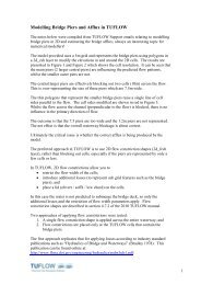
Pros and Cons of 1D and 2D Modeling - TUFLOW
Pros and Cons of 1D and 2D Modeling - TUFLOW
Pros and Cons of 1D and 2D Modeling - TUFLOW

You also want an ePaper? Increase the reach of your titles
YUMPU automatically turns print PDFs into web optimized ePapers that Google loves.
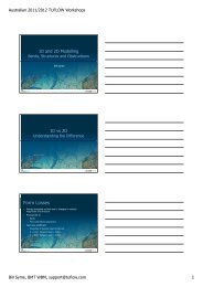
<strong>Pros</strong> <strong>and</strong> <strong>Cons</strong> <strong>of</strong> <strong>1D</strong> <strong>and</strong> <strong>2D</strong> <strong>Modeling</strong>, FMA Conference, San Diego, USA, Sep 2011<br />
<strong>Pros</strong> <strong>and</strong> <strong>Cons</strong> <strong>of</strong><br />
<strong>1D</strong> <strong>and</strong> <strong>2D</strong> <strong>Modeling</strong><br />
Bill Syme<br />
<strong>Pros</strong> <strong>and</strong> <strong>Cons</strong> <strong>of</strong><br />
<strong>1D</strong> <strong>and</strong> <strong>2D</strong> Modelling<br />
• Mathematical Reasons<br />
• Real-World Reasons<br />
2<br />
Bill Syme, BMT WBM, www.tuflow.com<br />
1
19 19 19 19 19 19<br />
-16 -16 -16 -16 -16 -16 -16 -16 -16<br />
<strong>Pros</strong> <strong>and</strong> <strong>Cons</strong> <strong>of</strong> <strong>1D</strong> <strong>and</strong> <strong>2D</strong> <strong>Modeling</strong>, FMA Conference, San Diego, USA, Sep 2011<br />
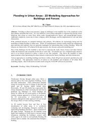
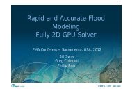
<strong>1D</strong> versus <strong>2D</strong><br />
Example <strong>of</strong> <strong>1D</strong> Network Model Output<br />
0<br />
28<br />
117<br />
1<br />
1<br />
10.44<br />
9.77<br />
11.52<br />
17<br />
1<br />
158 158 158<br />
158 158<br />
158<br />
11.52<br />
45<br />
1<br />
11.52<br />
233<br />
19<br />
11.52<br />
44<br />
137<br />
19 19 19<br />
11.50<br />
42 42 42 42 42 42 42 42 42<br />
3<br />
0<br />
10.44<br />
136 136 136 136 136 136 136 136 136<br />
242<br />
9.77<br />
34 34 34 34 34 34 34 34 34<br />
189<br />
4<br />
11.52<br />
206<br />
11.47<br />
379<br />
10.69<br />
Flow<br />
3<br />
223<br />
Flood Level<br />
11.53<br />
-<br />
<strong>1D</strong> versus <strong>2D</strong><br />
Example <strong>of</strong> Fully-<strong>2D</strong> Model Output<br />
Velocity Vector<br />
Bill Syme, BMT WBM, www.tuflow.com<br />
2
<strong>Pros</strong> <strong>and</strong> <strong>Cons</strong> <strong>of</strong> <strong>1D</strong> <strong>and</strong> <strong>2D</strong> <strong>Modeling</strong>, FMA Conference, San Diego, USA, Sep 2011<br />
<strong>1D</strong> versus <strong>2D</strong><br />
(<br />
(<br />
(<br />
(<br />
(<br />
(<br />
(<br />
(<br />
(<br />
( (<br />
(<br />
<strong>1D</strong> ~100 calculation points<br />
(<br />
<strong>2D</strong> ~10,000 calculation points<br />
(<br />
(<br />
(<strong>and</strong> longer simulation times)<br />
(<br />
(<br />
(<br />
(<br />
(<br />
(<br />
(<br />
(<br />
(<br />
(<br />
(<br />
(<br />
(<br />
(<br />
(<br />
(<br />
( (<br />
(<br />
(<br />
(<br />
(<br />
(<br />
(<br />
(<br />
(<br />
(<br />
(<br />
(<br />
(<br />
(<br />
(<br />
(<br />
(<br />
(<br />
( (<br />
(<br />
(<br />
5<br />
Key Physical Processes<br />
(What does your <strong>2D</strong> scheme solve?)<br />
How Velocity<br />
changes over time<br />
Inertia Term<br />
Coriolis<br />
Force<br />
Gravity<br />
Bed<br />
Resistance<br />
Atmospheric<br />
Pressure<br />
Viscosity<br />
(Turbulence)<br />
External<br />
Forces<br />
(Wind,<br />
Waves, …)<br />
∂v<br />
∂v<br />
∂v<br />
+ u + v + c<br />
∂t<br />
∂x<br />
∂<br />
y<br />
f<br />
∂h<br />
u + g<br />
∂<br />
y<br />
+ g v n<br />
2<br />
u<br />
2<br />
H<br />
+ v<br />
4<br />
3<br />
2<br />
⎛<br />
2 2<br />
v v ⎞ ∂p<br />
- ⎜ ∂ ∂ 1<br />
μ + ⎟<br />
+ =<br />
2 2<br />
F<br />
⎝ ∂ x ∂ y<br />
⎠<br />
ρ ∂<br />
y<br />
y<br />
What does your <strong>2D</strong> scheme need to solve to meet your objectives?<br />
6<br />
Bill Syme, BMT WBM, www.tuflow.com<br />
3
3<br />
<strong>Pros</strong> <strong>and</strong> <strong>Cons</strong> <strong>of</strong> <strong>1D</strong> <strong>and</strong> <strong>2D</strong> <strong>Modeling</strong>, FMA Conference, San Diego, USA, Sep 2011<br />
Bed Resistance<br />
• Manning’s equation most commonly used<br />
• Bed resistance dominant term where n is high<br />
• Compared with <strong>1D</strong><br />
• <strong>2D</strong> n values should be very similar for straight uniform flow<br />
(can be slightly higher due to no side friction)<br />
• based on calibrated <strong>2D</strong> models <strong>2D</strong> n values are similar or lower<br />
(lower where <strong>1D</strong> n values are artificially high due to sharp bends, etc)<br />
7<br />
Inertia<br />
23.2<br />
23.4<br />
23.2 23.2 23.2 23.2 23.2 23.2 23.2 23.2 23.2<br />
23.4 23.4 23.4 23.4 23.4 23.4 23.4 23.4 23.4<br />
23.6 23.6 23.6 23.6 23.6 23.6 23.6 23.6 23.6<br />
23.4 23.4 23.4 23.4 23.4 23.4 23.4 23.4 23.4<br />
23.2 23.2 23.2 23.2 23.2 23.2 23.2 23.2 23.2<br />
• 4 m/s<br />
• 20 m deep<br />
23.6 23.6<br />
23.6<br />
• 0.4m<br />
superelevation<br />
23.8 23.8 23.8 23.8 23.8 23.8 23.8 23.8 23.8<br />
24 24 24 24 24 24 24 24 24<br />
• <strong>1D</strong>:<br />
• Need additional<br />
losses<br />
(eg. higher n)<br />
• No superelevation<br />
24.4 24.4 24.4 24.4 24.4 24.4 24.4 24.4 24.4<br />
24.2<br />
23.8 23.8 23.8 23.8 23.8 23.8 23.8 23.8 23.8<br />
24<br />
23.8<br />
23.6 23.6 23.6 23.6 23.6 23.6 23.6 23.6 23.6<br />
23.4 23.4 23.4 23.4 23.4 23.4 23.4 23.4 23.4<br />
23 23 23 23 23 23 23 23 23<br />
22.8 22.8 22.8 22.8 22.8 22.8 22.8 22.8 22.8<br />
23.2 23.2 23.2 23.2 23.2 23.2 23.2 23.2 23.2<br />
22.6 22.6 22.6 22.6 22.6 22.6 22.6 22.6 22.6<br />
22<br />
2 4<br />
8<br />
Bill Syme, BMT WBM, www.tuflow.com<br />
4
<strong>Pros</strong> <strong>and</strong> <strong>Cons</strong> <strong>of</strong> <strong>1D</strong> <strong>and</strong> <strong>2D</strong> <strong>Modeling</strong>, FMA Conference, San Diego, USA, Sep 2011<br />
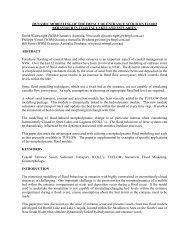
Right-Angled Bend<br />
<strong>1D</strong> vs <strong>2D</strong><br />
4<br />
(<br />
3<br />
3<br />
(<br />
1 <br />
( (<br />
1 2 2<br />
A<br />
0.5<br />
Water Surface Pr<strong>of</strong>iles (V = 2m/s)<br />
0.4<br />
Coarse <strong>2D</strong> Model<br />
<strong>1D</strong> Model<br />
<strong>1D</strong> Model<br />
evel (m)<br />
Water Le<br />
0.3<br />
02<br />
0.2<br />
0.1<br />
A<br />
0<br />
-0.1<br />
0 50 100 150 200 250 300 350 400 450<br />
Distance (m)<br />
9<br />
Viscosity<br />
Sub-Grid Scale Turbulence<br />
• Important where bed resistance term not<br />
dominant <strong>and</strong>/or<br />
rapid changes in velocity gradient<br />
• Low Manning’s n values <strong>and</strong>/or deep water<br />
• Flow constrictions<br />
• Smagorinsky formula preferred<br />
(varies coefficient based on velocity gradient)<br />
• Many <strong>2D</strong> schemes omit this term<br />
(Computationally intensive <strong>and</strong> difficult to solve)<br />
• Don’t artificially increase viscosity to<br />
stabilise models – distorts results<br />
10<br />
Bill Syme, BMT WBM, www.tuflow.com<br />
5
<strong>Pros</strong> <strong>and</strong> <strong>Cons</strong> <strong>of</strong> <strong>1D</strong> <strong>and</strong> <strong>2D</strong> <strong>Modeling</strong>, FMA Conference, San Diego, USA, Sep 2011<br />
<strong>1D</strong> Structures<br />
Contraction/Expansion Losses<br />
Simplified representation <strong>of</strong> complex flows<br />
11<br />
<strong>2D</strong> Structures<br />
No Contraction/Expansion Losses<br />
But need inertia/viscosity, ability to add fine-scale losses)<br />
12<br />
Bill Syme, BMT WBM, www.tuflow.com<br />
6
<strong>Pros</strong> <strong>and</strong> <strong>Cons</strong> <strong>of</strong> <strong>1D</strong> <strong>and</strong> <strong>2D</strong> <strong>Modeling</strong>, FMA Conference, San Diego, USA, Sep 2011<br />
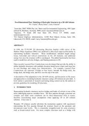
Eudlo Creek Hydraulic Investigations, Qld, 1998-2003<br />
Which Model?<br />
• Exhaustive Investigation<br />
• $4m damages claim<br />
• Physical Model (1:30 scale)<br />
• Four <strong>1D</strong> Models<br />
• HEC-RAS<br />
• MIKE 11<br />
• Rubicon<br />
• <strong>TUFLOW</strong> <strong>1D</strong><br />
• Three <strong>2D</strong> Models<br />
• FESWMS<br />
• MIKE 21<br />
• <strong>TUFLOW</strong><br />
13<br />
Eudlo Creek, Qld, 1998-2003<br />
Calibration<br />
11.15<br />
!11.06<br />
!(11.06<br />
• Three floods<br />
• 1983, 1992, 1999<br />
• One during study<br />
• Good data sets<br />
11.15<br />
!11.04<br />
!(<br />
9.88<br />
9.88<br />
(<br />
! 9.88<br />
10.38<br />
(<br />
!<br />
10.35<br />
10.69<br />
10.71<br />
(<br />
!!<br />
10.19<br />
10.25<br />
(<br />
!<br />
14 14<br />
Bill Syme, BMT WBM, www.tuflow.com<br />
7
<strong>Pros</strong> <strong>and</strong> <strong>Cons</strong> <strong>of</strong> <strong>1D</strong> <strong>and</strong> <strong>2D</strong> <strong>Modeling</strong>, FMA Conference, San Diego, USA, Sep 2011<br />
Pre-Duplication<br />
Post-Duplication<br />
15<br />
Eudlo Creek, Qld, 1998-2003<br />
Key Findings<br />
• Calibration<br />
(using st<strong>and</strong>ard parameters)<br />
• <strong>1D</strong> models poor<br />
(Could only reproduce recorded affluxes<br />
for the 3 calibration events using nonst<strong>and</strong>ard<br />
parameters – did not dissipate<br />
enough energy at bridge)<br />
• <strong>2D</strong> models performed well<br />
(only minor fine-tuning <strong>of</strong> parameters)<br />
• Physical model ?<br />
(once “rough” enough calibrated well)<br />
11.15<br />
!(11.06<br />
11.15<br />
1<br />
11.04<br />
(!!<br />
(<br />
!!<br />
(!<br />
10.38<br />
10.35<br />
9.88<br />
9.88<br />
10.69<br />
(!<br />
10.71<br />
10.19<br />
10.25<br />
(!!<br />
16<br />
Bill Syme, BMT WBM, www.tuflow.com<br />
8
<strong>Pros</strong> <strong>and</strong> <strong>Cons</strong> <strong>of</strong> <strong>1D</strong> <strong>and</strong> <strong>2D</strong> <strong>Modeling</strong>, FMA Conference, San Diego, USA, Sep 2011<br />
Eudlo Creek, Qld, 1998-2003<br />
Key Findings<br />
Flood Impacts<br />
• Performance in<br />
meeting objectives<br />
• <strong>1D</strong> models poor<br />
• Low confidence in results<br />
• <strong>2D</strong> models excellent<br />
• Slow to run (back then)<br />
• FESWMS: problematic<br />
• MIKE 21: limited <strong>2D</strong> structure<br />
representation<br />
• <strong>TUFLOW</strong>: numerous enhancements<br />
• Physical model good<br />
• Expensive<br />
• Very very slow turnover<br />
17<br />
Throsby Creek<br />
Newcastle (2006)<br />
• <strong>1D</strong><br />
• <strong>2D</strong><br />
• Sub <strong>and</strong><br />
super critical flow<br />
• 700 structures<br />
• 1,000 pipes, pits <strong>and</strong><br />
manholes<br />
• Complex overl<strong>and</strong> flows<br />
• Excellent calibration events<br />
18<br />
Bill Syme, BMT WBM, www.tuflow.com<br />
9
<strong>Pros</strong> <strong>and</strong> <strong>Cons</strong> <strong>of</strong> <strong>1D</strong> <strong>and</strong> <strong>2D</strong> <strong>Modeling</strong>, FMA Conference, San Diego, USA, Sep 2011<br />
Throsby Creek, NSW, 2006 - 2007<br />
<strong>1D</strong>/<strong>2D</strong> Model Development<br />
19<br />
Throsby Creek, NSW, 2006 - 2007<br />
<strong>1D</strong>/<strong>2D</strong> Model Results<br />
20<br />
Bill Syme, BMT WBM, www.tuflow.com<br />
10
<strong>Pros</strong> <strong>and</strong> <strong>Cons</strong> <strong>of</strong> <strong>1D</strong> <strong>and</strong> <strong>2D</strong> <strong>Modeling</strong>, FMA Conference, San Diego, USA, Sep 2011<br />
21<br />
Throsby Creek, Newcastle, NSW, 2006 (1990 Flood)<br />
22<br />
Bill Syme, BMT WBM, www.tuflow.com<br />
11
<strong>Pros</strong> <strong>and</strong> <strong>Cons</strong> <strong>of</strong> <strong>1D</strong> <strong>and</strong> <strong>2D</strong> <strong>Modeling</strong>, FMA Conference, San Diego, USA, Sep 2011<br />
Throsby Creek, Newcastle, NSW, 2006 (1990 Flood)<br />
23<br />
12.89<br />
( 3<br />
-0.08<br />
13.60<br />
(<br />
2<br />
0.05<br />
10.72<br />
(<br />
2<br />
028<br />
0.28<br />
12.06<br />
(<br />
2<br />
0.06<br />
13.86<br />
(<br />
3<br />
-0.17<br />
13.83<br />
(<br />
3<br />
-0.15<br />
12.97<br />
( 3<br />
-0.18<br />
12.62<br />
(<br />
3<br />
12.47<br />
-0.02<br />
(<br />
2<br />
0.14<br />
12.68 ( 2<br />
12.69<br />
(<br />
3<br />
0.12 -0.04<br />
13.15<br />
( 3<br />
-0.12<br />
12.70<br />
( 2<br />
0.18<br />
Throsby Creek, Newcastle, NSW, 2006 (1990 Flood)<br />
24 24<br />
Bill Syme, BMT WBM, www.tuflow.com<br />
12
<strong>Pros</strong> <strong>and</strong> <strong>Cons</strong> <strong>of</strong> <strong>1D</strong> <strong>and</strong> <strong>2D</strong> <strong>Modeling</strong>, FMA Conference, San Diego, USA, Sep 2011<br />
25<br />
26<br />
Bill Syme, BMT WBM, www.tuflow.com<br />
13
<strong>Pros</strong> <strong>and</strong> <strong>Cons</strong> <strong>of</strong> <strong>1D</strong> <strong>and</strong> <strong>2D</strong> <strong>Modeling</strong>, FMA Conference, San Diego, USA, Sep 2011<br />
Throsby Creek, NSW, 2006 – 2007<br />
June 2007<br />
• ~100 year flood<br />
(1 week after submitting 100 year flood maps!)<br />
• $700 million in damages<br />
• 5,000 cars written <strong>of</strong>f<br />
• Thous<strong>and</strong>s <strong>of</strong> homes inundated<br />
• >1,200 flood marks to verify model!<br />
• Field observations indicate an<br />
excellent comparison with modelling except...<br />
27<br />
June 2007 Throsby Creek Flood<br />
• Newcastle CBD<br />
• 1m deep – should be dry!<br />
• Outlet to harbour blocked by<br />
shipping container<br />
• New housing estate flooded<br />
• Should be dry<br />
• Two cars blocked main drain d/s<br />
• When blockages modelled, excellent<br />
comparisons resulted<br />
28<br />
Bill Syme, BMT WBM, www.tuflow.com<br />
14
<strong>Pros</strong> <strong>and</strong> <strong>Cons</strong> <strong>of</strong> <strong>1D</strong> <strong>and</strong> <strong>2D</strong> <strong>Modeling</strong>, FMA Conference, San Diego, USA, Sep 2011<br />
Casino Floodplain Management Study, NSW, 1999 – 2001<br />
CBD Levee Option<br />
Measures designed to alter the<br />
existing behaviour <strong>of</strong> the flood<br />
29<br />
Casino Floodplain Management Study, NSW, 1999 – 2001<br />
Switching to <strong>2D</strong> no longer made the community skeptical about modelling<br />
30<br />
Bill Syme, BMT WBM, www.tuflow.com<br />
15
<strong>Pros</strong> <strong>and</strong> <strong>Cons</strong> <strong>of</strong> <strong>1D</strong> <strong>and</strong> <strong>2D</strong> <strong>Modeling</strong>, FMA Conference, San Diego, USA, Sep 2011<br />
<strong>1D</strong> & Multiple <strong>2D</strong><br />
5m Grid<br />
<strong>1D</strong> In-bank<br />
5m Grid<br />
<strong>1D</strong> Culverts<br />
2m Grid<br />
<strong>1D</strong> In-bank<br />
31<br />
31<br />
Mapping <strong>1D</strong> Results<br />
• Mapping <strong>of</strong> <strong>1D</strong> results shows<br />
• Flow into hillside<br />
• Water levels don’t reflect<br />
lie <strong>of</strong> the l<strong>and</strong><br />
32<br />
Bill Syme, BMT WBM, www.tuflow.com<br />
16
<strong>Pros</strong> <strong>and</strong> <strong>Cons</strong> <strong>of</strong> <strong>1D</strong> <strong>and</strong> <strong>2D</strong> <strong>Modeling</strong>, FMA Conference, San Diego, USA, Sep 2011<br />
2002 – High Quality Flood Maps based on <strong>2D</strong> Modelling<br />
33<br />
Urban Areas – Buildings <strong>and</strong> Fences<br />
(<br />
(<br />
(<br />
(<br />
(<br />
(<br />
(<br />
(<br />
(<br />
(<br />
(<br />
(<br />
(<br />
(<br />
( (<br />
(<br />
(<br />
34<br />
Bill Syme, BMT WBM, www.tuflow.com<br />
17
<strong>Pros</strong> <strong>and</strong> <strong>Cons</strong> <strong>of</strong> <strong>1D</strong> <strong>and</strong> <strong>2D</strong> <strong>Modeling</strong>, FMA Conference, San Diego, USA, Sep 2011<br />
Modelling Fences!<br />
• Able to raise element sides<br />
• Element sides wet <strong>and</strong> dry<br />
• Layered parameters<br />
• eg. vary blockage<br />
<strong>and</strong> losses with height<br />
• Collapse element sides<br />
• Switch between u/s <strong>and</strong> d/s controlled<br />
weir flow<br />
35<br />
Collapsible Fences Animation<br />
36<br />
Bill Syme, BMT WBM, www.tuflow.com<br />
18
<strong>Pros</strong> <strong>and</strong> <strong>Cons</strong> <strong>of</strong> <strong>1D</strong> <strong>and</strong> <strong>2D</strong> <strong>Modeling</strong>, FMA Conference, San Diego, USA, Sep 2011<br />
Detailed Urban Models (2008)<br />
37<br />
Detailed Urban Models (2008)<br />
• 1,600 pipes / culverts<br />
• 900 pits (drains)<br />
• 600 manholes<br />
• 1.8 million wet cells at peak<br />
38<br />
Bill Syme, BMT WBM, www.tuflow.com<br />
19
<strong>Pros</strong> <strong>and</strong> <strong>Cons</strong> <strong>of</strong> <strong>1D</strong> <strong>and</strong> <strong>2D</strong> <strong>Modeling</strong>, FMA Conference, San Diego, USA, Sep 2011<br />
Modelling Blockages!?<br />
(These rails are recommended because they don’t collect debris...)<br />
39<br />
<strong>TUFLOW</strong> <strong>2D</strong> Layered Adjustments<br />
Blockage = 0%<br />
FLC = 0<br />
Blockage = 50%<br />
FLC = 0.5<br />
Blockage = 100%<br />
FLC = 0.8<br />
Blockage = 5%<br />
Form Loss Coeff = 0.1<br />
40<br />
Bill Syme, BMT WBM, www.tuflow.com<br />
20
<strong>Pros</strong> <strong>and</strong> <strong>Cons</strong> <strong>of</strong> <strong>1D</strong> <strong>and</strong> <strong>2D</strong> <strong>Modeling</strong>, FMA Conference, San Diego, USA, Sep 2011<br />
41<br />
Influence <strong>of</strong> Cell Size<br />
• Cell/Element Size(s)<br />
• Small enough to meet hydraulic objectiveses<br />
• Large enough to minimise run-times<br />
• Coarser than DEM<br />
• For a fixed grid model halving the cell size increases<br />
run-times by a factor <strong>of</strong> eight (8) – keep this in mind!<br />
42<br />
Bill Syme, BMT WBM, www.tuflow.com<br />
21
<strong>Pros</strong> <strong>and</strong> <strong>Cons</strong> <strong>of</strong> <strong>1D</strong> <strong>and</strong> <strong>2D</strong> <strong>Modeling</strong>, FMA Conference, San Diego, USA, Sep 2011<br />
43<br />
44<br />
Bill Syme, BMT WBM, www.tuflow.com<br />
22
<strong>Pros</strong> <strong>and</strong> <strong>Cons</strong> <strong>of</strong> <strong>1D</strong> <strong>and</strong> <strong>2D</strong> <strong>Modeling</strong>, FMA Conference, San Diego, USA, Sep 2011<br />
45<br />
Fine-Scale Modelling<br />
<strong>TUFLOW</strong> FV Flexible Mesh Engine<br />
UK EA benchmarking to flume test – smallest element a 2½ cm triangle<br />
46<br />
Bill Syme, BMT WBM, www.tuflow.com<br />
23
<strong>Pros</strong> <strong>and</strong> <strong>Cons</strong> <strong>of</strong> <strong>1D</strong> <strong>and</strong> <strong>2D</strong> <strong>Modeling</strong>, FMA Conference, San Diego, USA, Sep 2011<br />
<strong>2D</strong> or 3D?<br />
<strong>2D</strong><br />
3D<br />
23 cm 30 cm<br />
47<br />
47<br />
Conclusions<br />
• <strong>1D</strong> models <strong>of</strong>fer a better solution<br />
• where <strong>2D</strong> resolution is too coarse<br />
• for pipes, manholes <strong>and</strong> small structures<br />
• <strong>1D</strong> requires more judgment<br />
(therefore greater uncertainty)<br />
• <strong>1D</strong> solutions vary (eg. steady vs unsteady)<br />
• <strong>1D</strong> solutions are<br />
• very fast<br />
• a poor approximation <strong>of</strong> complex (non-unidirectional) flows<br />
48<br />
Bill Syme, BMT WBM, www.tuflow.com<br />
24
<strong>Pros</strong> <strong>and</strong> <strong>Cons</strong> <strong>of</strong> <strong>1D</strong> <strong>and</strong> <strong>2D</strong> <strong>Modeling</strong>, FMA Conference, San Diego, USA, Sep 2011<br />
Conclusions<br />
• <strong>2D</strong> or <strong>1D</strong>/<strong>2D</strong> models <strong>of</strong>fer significant gains<br />
• in accuracy <strong>of</strong> flood modeling, risk <strong>and</strong> flood impact predictions<br />
• in stakeholder underst<strong>and</strong>ing <strong>and</strong> acceptance<br />
• but are slow in comparison to <strong>1D</strong> only<br />
• Underst<strong>and</strong> your s<strong>of</strong>tware<br />
• Different <strong>2D</strong> solutions vary significantly in performance<br />
• Make sure your <strong>2D</strong> scheme solves the key physical processes needed<br />
• Models still need to be<br />
• Calibrated where possible<br />
• Quality Controlled: Garbage In / Garbage Out<br />
49<br />
Eudlo Creek, 1952<br />
Thank You<br />
Bill Syme, BMT WBM, www.tuflow.com<br />
25