Dummy Variables and Omitted Variable Bias

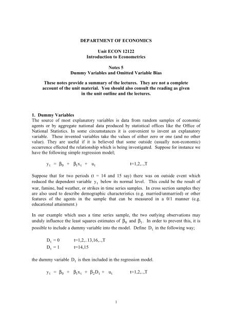
2. Omitted Variable BiasSo far we have assumed that the linear regression model is the correct specification of therelationship between the dependent and the explanatory variables. But suppose it is not.If it is not the correct specification, the model is then termed “mis-specified”. There arenumber of kinds of mis-specification and each kind has different consequences forestimation and hypothesis testing. Here we will deal with one of the most commonkinds; the omission of an explanatory variable.The linear regression model can, of course, contain a number of explanatory variables.The number is limited by the number of observations. In general, the number ofobservations should be several times greater than the number of explanatory variables.Nevertheless, it is still possible for an explanatory variable to be omitted either becauseits influence on the dependent variable is unknown or because it is difficult or impossibleto find data on such a variable. We are interested in the consequences for the leastsquares estimators of this omission.We will take the simplest possible case. Suppose the true model is;y t =a 1 x t + 2 z ta + u tt=1,2,… T (2)where u t is an unobserved random variable, E( ut⏐x t , z t ) = 0.However for whatever reason the second explanatory variable z t is omitted and theeconometrician assumes that the correct model is;y t =a 1 x t + u tt=1,2,… T (3)The least squares estimate of a 1 will beâ 1 =∑ x y∑ xt t2t(4)What are the properties of â 1?As before (see Notes 3), we take the expression for â 1 (4) and substitute for y t . On thisoccasion we substitute not from the false model (3), but from the true model (2). Thusâ 1 =∑ x (a x + a z + ut1t∑ x2 t t2t)= a 1 +a ∑ x z2∑ xt t2t+∑ x u∑ xt t2t(5)We now wish to examine whether â 1 is biased or unbiased. To do this we takeexpectations of (5).⎛E( â 1 ) = E( a 1 ) + E⎜a2∑x z⎝ ∑ xt t2t⎞ ⎛⎟ + E⎜∑x tu2⎠ ⎝ ∑ x tt⎞⎟⎠4

e positive for theoretical reasons as well), the sign of the omitted variable bias is, in thisexample, negative.The consequence of this bias is that the estimated coefficient of unemployment in (8) willbe smaller that it should be. You will be able to confirm that the least squares estimate ofa 1 in (8) is smaller (a larger negative number) than −0.509. The comparatively largenegative effect of unemployment on wages which was found by estimating (8) is nowconsiderably reduced.In addition the estimated coefficient of unemployment (unlike that of inflation) is notsignificant in (9). We can tell this by calculating the absolute value of its t ratio;0.509/0.501 = 1.016This has a t distribution with 19 degrees of freedom. We cannot reject the null hypothesisthat the coefficient of unemployment is zero (for the 95% critical value see above).Notice that the standard error here (0.501) is comparatively large. The 95% confidenceinterval goes from −1.56 to 0.54. This includes some relatively large negative numbersas well as some smaller positive ones. It is still possible that there maybe a fairlysubstantial effect of unemployment on percentage wage changes. It would be unwise toconclude from these estimates that there is no unemployment effect. (see Tests ofSignificance in Notes 4.)It is interesting to compare the results in (9) with those when the dummy variable is2included as in (1). Equation (1) has the higher R and thus (1) is the better “fit” to thedata. The estimates of the unemployment coefficient differ by a fairly wide margin(− 1.709 , − 0.509). Such a difference could have important policy implications.Which is the better equation will depend on a number of factors, such as the pattern of theresiduals, which we have not discussed. However it would seem that there are goodtheoretical reasons for including retail price inflation in the regression. It appears tocapture whatever political effects occurred in 1975 and 1980 (the residuals in (9) for 1975and 1980 are not particularly large). Where an economic explanatory variable isavailable it is to be preferred to the “ad hoc” dummy variable. Dummy variables shouldreally be reserved for events which are completely non-economic. Thus I would preferthe estimates in (9) to those in (1).One problem with (9), concerns causation. Was price inflation driving up wages in thisperiod, or were wage changes driving up prices? Or were both variables influencing eachother? The answers to these and other questions will be dealt with in subsequent units inEconometrics.David WinterApril 20007