Bivariate or joint probability distributions

1
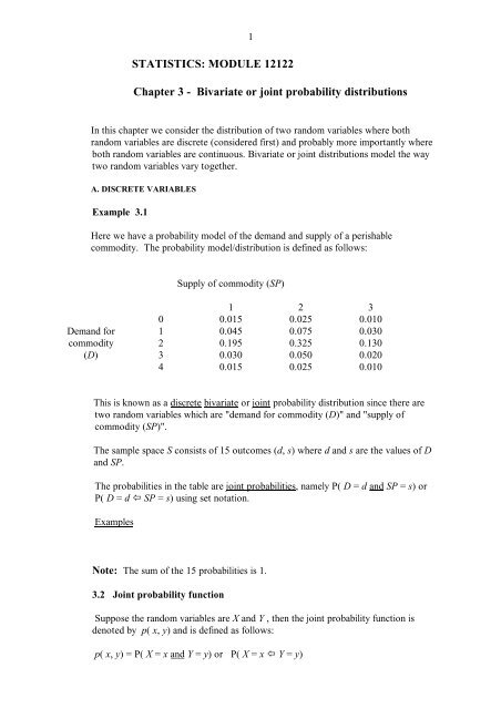
STATISTICS: MODULE 12122
Chapter 3 - Bivariate or joint probability distributions
In this chapter we consider the distribution of two random variables where both
random variables are discrete (considered first) and probably more importantly where
both random variables are continuous. Bivariate or joint distributions model the way
two random variables vary together.
A. DISCRETE VARIABLES
Example 3.1
Here we have a probability model of the demand and supply of a perishable
commodity. The probability model/distribution is defined as follows:
Supply of commodity (SP)
1 2 3
0 0.015 0.025 0.010
Demand for 1 0.045 0.075 0.030
commodity 2 0.195 0.325 0.130
(D) 3 0.030 0.050 0.020
4 0.015 0.025 0.010
This is known as a discrete bivariate or joint probability distribution since there are
two random variables which are "demand for commodity (D)" and "supply of
commodity (SP)".
The sample space S consists of 15 outcomes (d, s) where d and s are the values of D
and SP.
The probabilities in the table are joint probabilities, namely P( D = d and SP = s) or
P( D = d ï SP = s) using set notation.
Examples
Note: The sum of the 15 probabilities is 1.
3.2 Joint probability function
Suppose the random variables are X and Y , then the joint probability function is
denoted by p( x, y) and is defined as follows:
p( x, y) = P( X = x and Y = y) or P( X = x ï Y = y)

∑ ∑ , = 1.
Also p( x y)
x
y
2
3.3 Marginal probability distributions
The marginal distributions are the distributions of X and Y considered separately
and model how X and Y vary separately from each other. Suppose the probability
functions of X and Y are p
X ( x)
and pY ( y)
respectively so that
p
X ( x)
= P(X = x) and p ( y)
Also ∑ p
X ( x)
= 1 and pY
( y)
x
∑ = 1.
y
Y
= P(Y = y)
It is quite straightforward to obtain these these from the joint probability distribution
p x p x , y p y p x , y
since
X ( ) = ∑ ( ) and
Y ( ) = ∑ ( )
y
In regression problems we are very interested in conditional probability distributions
such as the conditional distribution of X given Y = y and the conditional distribution
of Y given X = x
x
3.4 Conditional probability distributions
The conditional probability function of X given Y = y is denoted by p( x y)
is defined as
p( x y ) = P( X x Y y)
= = =
( = = )
P( Y = y)
P X x and Y y
=
( , )
( y)
p x y
whereas the conditional probability function of Y given X = x is denoted by p( y x)
and defined as
p( y x ) = P( Y y X x)
= = =
( = = )
P( X = x)
P Y y and X x
=
p
Y
( , )
( x)
p x y
p
X
3.5 Joint probability distribution function
The joint (cumulative) probability distribution function (c.d.f.) is denoted by F(x, y)
and is defined as
F(x, y) = P( X ó x and Y ó y) and 0 ó F(x, y) ó 1
The marginal c.d.f ’s are denoted by FX ( x)
and F ( y)
F
X ( x)
= P( X ó x) and F ( y)
(see Chapter 1, section 1.12 ).
Y
= P( Y ó y)
Y
and are defined as follows

3
3.6 Are X and Y independent?
If either (a) F(x, y) = FX ( x)
. FY ( y)
or (b)p(x, y) = p
X ( x)
. pY
( y)
then X and Y are independent random variables.
Example 3.2 The joint distribution of X and Y is
X
-2 -1 0 1 2
Y 10 0.09 0.15 0.27 0.25 0.04
20 0.01 0.05 0.08 0.05 0.01
(a) Find the marginal distributions of X and Y.
(b) Find the conditional distribution of X given Y =20.
(c) Are X and Y independent?
B. CONTINUOUS VARIABLES
3.7 Joint probability density function
The joint p.d.f. is denoted by f (x, y) (where f ( x , y)
≥ 0 all x and y) and defines
a probability surface in 3 dimensions. Probability is a volume under this surface and
the total volume under the p.d.f. surface is 1 as the total probability is 1 i.e.
∞
∞
( , )
∫ ∫ f x y dx dy = 1
−∞
−∞
y=
d x=
b
and P( a ó X ó b and c ó Y ó d ) = ( , )
∫
∫
y=
c x=
a
f x y dx dy
As before with discrete variables, the marginal distributions are the distributions of
X and Y considered separately and model how X and Y vary separately from each other.
Whereas with discrete random variables we speak of marginal probability functions,
with continuous random variables we speak of marginal probability density functions.
Example 3.3
An electronics system has one of each of two different types of components in joint
operation. Let X and Y denote the random lengths of life of the components of type 1
and 2, respectively. Their joint density function is given by
( x y)
/
f ( x , y) = ⎛ x e x ; y
⎝ ⎜ 1 ⎞ ⎠ ⎟ − + 2
> 0 > 0
8
= 0
otherwise

4
Example 3.4
The random variables X and Y have a bivariate normal distribution if
( )
−
f x, y = ae b
where
a=
2π σ σ 1−
ρ
X
1
Y
2
and
b =
1
2
( − ρ )
2 1
⎡ ⎛ x − µ ⎞ ⎛
X
x − µ ⎞ ⎛
X
y − µ ⎞ ⎛
Y
y − µ
⎢ ⎜ ⎟ − 2ρ⎜
⎟ ⎜ ⎟ + ⎜
⎣⎢
⎝ σ
X ⎠ ⎝ σ
X ⎠ ⎝ σ
Y ⎠ ⎝ σ
Y
2 2
Y
⎞
⎟
⎠
⎤
⎥
⎦⎥
where −∞< x

3.9 Conditional probability density functions
The conditional p.d.f of X given Y = y is denoted by f ( x y)
and
defined as f ( x y ) = f ( x Y y)
= =
5
( , )
( y)
f x y
whereas the conditional p.d.f of Y given X = x is denoted by f ( y x)
and
defined as f ( y x ) = f ( y X x)
= =
f
Y
( , )
( x)
f x y
f
X
3.10 Joint probability distribution function
As in 3.5 the joint (cumulative) probability distribution function (c.d.f.) is denoted by
F(x, y) and is defined as F(x, y) = P( X ó x and Y ó y) but F(x, y) in the continuous
case is the volume under the p.d.f. surface from X = −∞ to X = x and from Y = −∞ to
Y = y, so that
F( x y)
v=
y
∫
u=
x
, = ( , )
v=−∞
∫
u=−∞
f u v du dv
The marginal c.d.f. ‘s are defined as in 3.5 and can be obtained from the joint
distribution function F(x, y) as follows:
F
F
X ( x)
= F( x y MAX )
Y ( y)
= F( x y)
, where y MAX
is the largest value of y and
MAX , where x MAX
is the largest value of x.
3.11 Important connections between the p.d.f ‘s and the joint c.d.f.’s.
(i) The joinf p.d.f. f (x, y) =
( , )
∂
2 F x y
∂x∂y
(ii) The marginal p.d.f’s can be obtained from the marginal c.d.f.’s as follows:
the marginal p.d.f. of X = f ( x)
X
=
the marginal p.d.f. of Y = f ( y)
Y
=
dF
X
dx
dF y
Y
dy
( x)
( )
or F ′ ( x)
X
,
or F ′ ( y)
Y
3.12 Are X and Y independent?
X and Y are independent random variables if either
(a) F(x, y) = FX ( x)
FY
( y)
; or

(b) f(x, y) = f
X ( x)
f ( y)
Y
; or
6
(c) f ( x y ) = function of x only or equivalently f ( y x ) = function of y only
Example 3.5 The joint distribution function of X and Y is given by
F x y y x 2
⎛ ⎞
2
( , ) =
3 ⎜ + x⎟ ⎝ 2 ⎠
0≤ x,
y ≤1
= 0 otherwise
(i) Find the marginal distribution and density functions.
(ii) Find the joint density function.
(iii) Are X and Y independent random variables?
Example 3.6
X and Y have the joint probability density function
2
8x
f ( x, y)
= 1≤ x,
y≤
2
3
7y
(a) Derive the marginal distribution function of X.
(b) Derive the conditional density function of X given Y = y
(c) Are X and Y independent?
Given:
Given:
Joint density fn. f (x ,y) Joint distribution fn. F(x, y)
⏐ Integrate w.r.t ⏐ Differentiate (partially)
⏐ x and y ⏐ w.r.t. x and y
↓
↓
Joint distribution fn. F(x, y) Joint density fn. f (x, y)
v=
y
∫
v=−∞
u=
x
∫
u=−∞
( , )
f u v du dv
∂
2 F
∂x∂y .

Example 3.6(b) and (c)
7
Solution From 3.9 the conditional p.d.f of X given Y = y is denoted by f ( x y)
and
defined as f ( x y ) = f ( x Y y)
= =
( , )
( y)
f x y
and Y and fY ( y)
is the marginal p.d.f. of Y. We know f ( x y)
find f ( y)
Y
.
There are two ways you can find f ( y)
f
Y
where f ( x , y)
is the joint p.d.f. of X
x
, = 8 7y
2
3
so we need to
Y
. The first way involves integration and the
second way involves differentiation. I will do both ways to show you how to use the
different results we have here but you should always choose the way you find easiest i.e
you would not be expected to find fY ( y)
both ways in any assessed work .
Method 1
∞
From 3.8 fY ( y)
= ∫ f ( x , y)
dx so f ( y)
−∞
Y
=
2
2
8x
∫ 3
7y
dx =
1
8
y
2
7 3 2
∫ x dx =
1
2
3
8 ⎡ x ⎤
3 ⎢
7y
⎣ 3
⎥ =
⎦
1
=
8
7y
3
3
⎡2
⎢
⎣ 3
−
1⎤
⎥
3
= 8
⎦ 7y
3
⎡7
⎣
⎢3
⎤
⎦
⎥ = 8
y
3 3
Method 2
From 3.11 f ( y)
Y
=
dF
Y
( y)
dy
From 3.10 FY ( y)
= F( x y)
F
F
where F ( y)
MAX , where x MAX
Y ( y)
= F( 2, y)
and from part (a), F( x y)
( y)
Hence f ( y)
4
21 2 1 ⎛
1 1 ⎞
⎜ −
2 ⎟ = 4 ⎛
⎝ y ⎠ 3 1 1 ⎞
⎜ −
2 ⎟
⎝ y ⎠
3
2, = ( − )
Y
= d ⎛ 4 ⎛
dy 3 1 1 ⎞⎞
⎜ ⎜ −
2
⎟⎟ = 4 ⎛ 2 ⎞
⎜ 3 ⎟ =
⎝ ⎝ y ⎠⎠
3 ⎝ y ⎠
Y
is the marginal c.d.f of Y.
is the largest value of x, so
4
21
3
, = ( x − )
8
3y
3
hence F ( y)
⎛
1 ⎜1−
⎝
1 ⎞
2 ⎟ so
y ⎠
Y
= 4 ⎛
3 1 1 ⎞
⎜ −
2 ⎟ .
⎝ y ⎠
as with method 1.
Now therefore the conditional density function of X given Y = y , f ( x y)
is given by
So ( )
f
f ( x y ) = ( x,
y )
f ( y)
Y
=
⎛ 8x
⎜
⎝ 7y
⎛ 8
⎜
⎝ 3y
2
3
3
⎞
⎟
⎠
⎞
⎟
⎠
= 3 x
7
f x y = 3 3
x
7
1 ó x ó 2 and 1 ó y ó 2
= 0 otherwise
(c) Now f ( x y)
is a function of x only, so using result 3.12(c), X and Y are independent.
Notice also that f ( x y ) = f
X ( x)
which you would expect if X and Y are independent.
3

3.13 Expectations and variances
8
Discrete random variables
r
r
r
r
( ) = ∑ ∑ ( , ) = ∑ x ∑ p( x , y)
= x p
X ( x)
E X x p x y
x
y
x
r
r
r
r
( ) = ∑ ∑ ( , ) = ∑ y ∑ p( x , y)
= y pY
( y)
E Y y p x y
Examples
x
y
y
y
x
∑ r =1,2.....
x
∑ r =1,2....
y
2 2
Hence Var(X) = E( X ) − ( E( X ))
, Var(Y) = E( Y ) ( E( Y
)
Continuous random variables
∞
∞
r r r
( ) ∫ ∫ ( ) ∫ X ( )
− etc.
2 2
E X = x f x , y dx dy = x f x dx r = 1, 2 .....
−∞ −∞
∞
∞
r r r
( ) ∫ ∫ ( ) ∫ Y ( )
E Y = y f x , y dx dy = y f y dy r = 1, 2 .....
Examples
−∞ −∞
∞
−∞
∞
−∞
3.14 Expectation of a function of the r.v.'s X and Y
Continuous X and Y
Discrete X and Y
∞
∞
∫ ∫
E[ g( X, Y)] = g( x, y) f ( x, y)
dxdy
−∞ −∞
∞
∞
e . g . ⎡
E X ⎤ x
⎣
⎢ Y ⎦
⎥ = ∫ ∫
y f ( x, y)
dxdy
E[XY] =
−∞ −∞
∞
∞
∫ ∫
−∞ −∞
xy f ( x , y ) dxdy .
3.15 Covariance and correlation
Covariance of X and Y is defined as follows : Cov (X,Y) = σ XY
= E(XY) - E(X)E(Y).
Notes
(a) If the random variables increase together or decrease together, then the covariance
will be positive, whereas if one random variable increases and the other variable
decreases and vice-versa, then the covariance will be negative.
(b) If X and Y are independent r.v's, then E(XY) = E(X)E(Y) so cov(X, Y) = 0.
However
if cov(X,Y) = 0, it does not follow that X and Y are independent unless X and Y are

9
Normal r.v's.
Correlation coefficient = ρ = corr(X,Y) = Cov ( X , Y ) .
σ
Xσ
Y
Note
(a) The correlation coefficient is a number between -1 and 1 i.e. -1 ó ρ ó 1
(b) If the random variables increase together or decrease together, then ρ
will be positive, whereas if one random variable increases and the other variable
decreases and vice-versa, then ρ will be negative.
(c) It measures the degree of linear relationship between the two random variables X
and Y , so if there is a non-linear relationship between X and Y or X and Y are
independent random variables, then ρ will be 0.
You will study correlation in more detail in the Econometric part of the course with
David Winter.
Example 3.7 In Example 3.2 are X and Y correlated?
Solution Below is the joint or bivariate probability distribution of X and Y:
X
-2 -1 0 1 2
Y 10 0.09 0.15 0.27 0.25 0.04
20 0.01 0.05 0.08 0.05 0.01
The marginal distributions of X and Y are
x -2 -1 0 1 2 Total
p
X
x
0.10 0.20 0.35 0.30 0.05 1.00
P(X =x) or ( )
and
P(Y = y) or ( )
y 10 20 Total
pY y
0.8 0.20 1.00
Example 3. 8 In Example 3.6
(i) Calculate E(X), Var(X), E(Y) and cov(X,Y).
(ii) Are X and Y independent?
3.14 Useful results on expectations and variances
(i) E( aX + bY) = aE( X) + bE( Y)
where a and b are constants.

10
(ii) Var( aX + bY) = a Var( X) + b Var( Y) + 2ab cov( X, Y).
Result (i) can be extended to any n random variables X 1
, X 2
,......., X n
E a X + a X + ....... + a X = a E X + a E X + ........ + a E X
( ) ( ) ( ) ( )
1 1 2 2 n n 1 1 2 2
n n
When X and Y are independent, then
(iii) Var( aX + bY) = a 2 Var( X) + b 2 Var( Y)
= so cov( X, Y ) = 0
(iv) E( XY ) E( X) E( Y )
Results (iii) and (iv) can be extended to any n independent random variables
X 1
, X 2
,......., X n
(iii)* Var( a X a X ....... a X )
+ + + =
1 1 2 2
n
n
2
2
( ) + ( ) + ........ + ( )
2
a Var X a Var X a Var X
1
1 2
(iv)* E( X X ..... X ) = E( X ). E( X )........
E( X )
1 2 n
1 2
n
2
n
n

11
3.15 Combinations of independent Normal random variables
Suppose X
X
2
2
2
~ N ( µ , σ ) , X ~ N( µ , σ ) , X ~ N ( µ , σ ) ,.........and
1 2 2
2 2 2
3 3 3
~ N ( µ , σ 2 ) X 1
, X 2
,......., X n
are independent random variables, then if
n n n
Y = a1 X1 + a2 X2 + a3 X3 + ..... + a n
X n
where a 1
, a 2
..... a n
are constants,
2 2 2 2 2 2
Y ~ N( a µ + a µ + a µ + ..... + a µ , a σ + a σ + ..... + a σ )
1 1 2 2 3 3 n n 1 1 2 2
n n
∑
i.e. Y ~ N( a µ , a σ 2 ).
∑
i i i i

12
In particular, suppose X 1
, X 2
..... X n
form a random sample from a Normal
population with mean µ and variance σ 2 ,
2 2 2 2
µ = µ = µ = ..... = µ = µ and σ = σ = ..... = σ = σ .
1 2 3 n
1
∑
Y ~ N( a µ , a
2 σ
2 ).
i
∑
i
2
n
Further, suppose that a = a = a = ..... = a =
1 2 3
n
1
n
then Y = X + X + X
1 2
...
n
n
=
X
and X ~ N( µ , σ 2 ) .
n