are irrational expectations rational? David Demery Nigel W. Duck1 ...

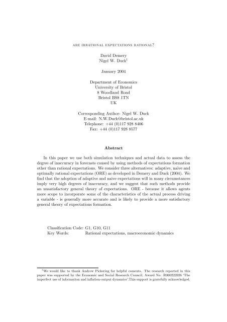
are irrational expectations rational?David DemeryNigel W. Duck 1January 2004Department of EconomicsUniversity of Bristol8 Woodland RoadBristol BS8 1TNUKCorresponding Author: Nigel W. DuckE-mail: N.W.Duck@bristol.ac.ukTelephone: +44 (0)117 928 8406Fax: +44 (0)117 928 8577AbstractIn this paper we use both simulation techniques and actual data to assess thedegree of inaccuracy in forecasts caused by using methods of expectations formationother than rational expectations. We consider three alternatives: adaptive, naive andoptimally rational expectations (ORE) as developed in Demery and Duck (2004). Wefind that the adoption of adaptive and naive expectations will in many circumstancesimply very high degrees of inaccuracy, and we suggest that such methods providean unsatisfactory general theory of expectations. ORE - because it allows agentsmore scope to incorporate some of the characteristics of the actual process drivinga variable - is generally more accurate and is likely to provide a more satisfactorygeneral theory of expectations formation.Classification Code: G1, G10, G11Key Words: Rational expectations, macroeconomic dynamics1 We would like to thank Andrew Pickering for helpful coments. The research reported in thispaper was supported by the Economic and Social Research Council, Award No. R000223926 ‘Theimperfect use of information and inflation-output dynamics’.This support is gratefully acknowledged.

Are Irrational Expectations Rational? 11 IntroductionDemery and Duck (2004) note an early and subsequently neglected theoreticalcriticism of rational expectations (RE) and use it to develop analternative model of expectations formation which may help explain someof the empirical failings of macroeconomic models which incorporate RE.The early criticism was expressed in Feige and Pearce (1976) and Buiter(1980) who argued that an agent’s decision about how to form expectationsshould be analyzed like any other economic decision, from a choice-theoreticframework in which the agent weighs up the costs and benefits of formingexpectations in different ways. 1In the framework constructed in Demery and Duck (2004) the variableto be forecast is either an aggregate variable or a component of that aggregate.Each component is influenced by two processes, one of which iscommon to all components and the other of which is idiosyncratic. Withinthis framework agents can choose the number of components of the aggregatethey observe and hence the size of their information set. Once theyhave chosen their information set, they will fully exploit it when formingexpectations. The greater the size of the information set, the more accuratetheir forecasts will be but so too will the costs of acquiring, maintaining andinterpreting their information set. On plausible assumptions, in many situationsa rational agent will choose not to acquire all the available informationand will form expectations that depart from fully rational expectations butwhich Demery and Duck term optimally rational expectations, ORE. Demeryand Duck (2001, 2004) show that such expectations can explain someof the empirical failures of macroeconomic models which incorporate rationalexpectations.In this paper we address the problem of whether the losses involved innot forming rational expectations are likely to be high. We consider fouralternative methods of forming expectations: RE, ORE, adaptive expectations,and naïve expectations. We attempt, through a mixture of simulationand empirical evidence, to obtain estimates of how serious any departuresfrom RE are likely to be in the alternative three cases. In the first partof the paper we present our framework for analyzing different methods ofexpectations formation. In the second we present evidence from some simplesimulations about the loss of accuracy involved in forecasting methodswhich depart from RE. In the third we consider the same question but using1 Buiter (1980) makes the point as follows: ‘[T]he term rational ... expectations oughtto be reserved for forecasts generated by a rational, expected utility maximising decisionprocess in which the costs of acquiring, processing and evaluating additional informationare balanced against the anticipated benefits from further refinement of forecasts’ (p.35).Feige and Pearce (1976) made the same point, arguing that ‘[R]ational expectationsmodels offer the theoretical appeal of greater consistency with the economist’s paradigm ofrational behaviour in a world of negligible information costs; however, they avoid speakingto the empirical issue of selecting a particular information set’ (p.518).

Are Irrational Expectations Rational? 2actual data on inflation rates in 10 US cities.Our main conclusions are that the naïve and adaptive methods of expectationsformation can lead to such high losses that - even if one were toignore other well-known objections to them - they cannot provide a theoreticallysatisfactory general theory of expectations formation. In essencethe reason for this is that neither method provides a sufficiently subtle wayfor agents to incorporate information about the true nature of the processdriving the variable they are forecasting. In some circumstances - notablywhen the common and idiosyncratic processes are very different but wherethey contribute equally to movements in the variable being forecast - OREtoo can lead to a high degree of inaccuracy but even in these cases the agentscan reduce the inaccuracy by acquiring more series. More generally, OREbased on a small number of series appears to deliver results that are closeto the accuracy delivered by RE.2 General frameworkIn many macroeconomic settings it is natural to think of variables as beingeither an aggregate variable or a component of an aggregate. Let x t representthe aggregate or average variable at time t, andletx j,t represent the j thcomponent of that aggregate. So, for example, x t might represent aggregatereal output or income, and x j,t the real output or income of a particularindividual or firm. Or x t might represent aggregate nominal spending andx j,t the nominal spending of one individual. Or, again, x t might representthe aggregate price level and x j,t the price of a particular good. The generalrelationship between x t and x j,t can be writtenNXx t = w j x j,tj=1where w j is the weight attached to x j,t in the construction of the aggregate,and N is the number of components. In what follows, merely to avoidunnecessary notational complications, we shall assume that all variableshave equal weight in the construction of the aggregate and sox t = 1 NNXx j,tj=1The distinction between x t and x j,t allows us to split the behaviour ofthe variable x j,t into two componentsx j,t ≡ x t +(x j,t − x t )From this perspective the behaviour of the variable x j,t canbeseenastheresult of two distinct forces or processes. The first - the process driving x t

Are Irrational Expectations Rational? 3- is aggregate in nature and is common to all components of the aggregate.The second - the process driving (x j,t − x t ) - is idiosyncratic. In their nature,the idiosyncratic processes sum to zero across j.We shall assume that both x t and (x j,t − x t ) are stationary and areuncorrelated with each other. We represent the stationary, aggregate component,x t , in the following invertible moving-average error form:T 1Xx t = α(L)ε t = α i ε t−i (1)i=0where α(L) is a polynomial in the lag operator with α 0 =1and ε is aGaussian white-noise error process with zero mean and variance σ 2 ε. 2Similarly, we represent the stationary, idiosyncratic component, (x j,t − x t ),in the following invertible moving-average error form:T 2Xx j,t − x t = γ(L)u j,t = γ i u j,t−i (2)i=0where γ(L) is a polynomial in the lag operator with γ 0 =1;andu j,t is aGaussian white-noise error process with zero mean and variance σ 2 u. Weassume that u j,t is uncorrelated with ε t at all leads and lags, and is uncorrelatedwith u j−v,t−k for all values of v and k other than zero. 3 In what followswe assume that at least some of the αs aredifferent from the equivalent γs.We also assume that T 1 = T 2 = T . 4It follows that x j,t can be represented as the sum of two moving-averageerror processes:TXTXx j,t = α i ε t−i + γ i u j,t−i (3)i=0i=0To fix our timing convention, we assume that, for all v ≥ 0, ε t+v and u j,t+vcannot be known at t, whereas all other values of ε t+v and u j,t+v are feasibleelements of any agent’s information set at period t. Wemeanbythisthatno expenditure of resources would allow the agent to know the value of ε t oru j,t in period t, whereas,withsomefinite expenditure, agents can acquireknowledge of past values of ε t or u j,t .Consider now how an agent might form expectations about x j,t or x t .We shall restrict ourselves to one-period ahead forecasts.2 By the Wold representation theorem, covariance stationary variables have movingaverageerror representations. We have assumed a finite-order moving-average processbut this is not essential.3 Equation (2) implies that P Nuj,t−i =0. Our assumption about the lack of correlationbetween u j,t and u j−v,t for all v requires that N is ‘large’.4 If T 1 6= T 2 , then whichever is the lower-order process can always be redefined toj=1include the required extra number of terms attached to zero coefficients.

Are Irrational Expectations Rational? 42.1 Rational expectationsBy rational expectations we mean that each agent is assumed to conditiontheir expectation on the full information set. In the present context thismeans that agents use the information set consisting of the separate historiesof ε t and of u j,t for j =1, 2,...N. These separate histories, together withpresumed knowledge of the structure of the economy represented by the αand γ parameters, allow us to write the one-period-ahead RE forecast of x j,tand x t asE REj,t−1x j,t =E REj,t−1x t =TXTXα i ε t−i + γ i u j,t−ii=1i=1TXα i ε t−ii=1The expectational errors will be respectively,R REj,tAR REj,t≡ x j,t − E REj,t−1x j,t = ε t + u j,t≡ x t − E REj,t−1x t = ε tBoth of these are white noise errors with variances σ 2 ε + σ 2 u,andσ 2 ε respectively.2.2 Naïve expectationsBy naïve expectations we mean that agents expect that the value any variabletakes next period will equal its most recently observed value. So, in thetwo cases we have here, the naïve expectations can be written,Ej,t−1x NA j,t = x j,t−1E NAj,t−1x t = x t−1The expectational errors in this case will beTXRj,t NA ≡ x j,t − Ej,t−1x NA j,t = ε t + (α i − α i−1 ) ε t−ii=1TX ¡ ¢+ γi − γ i−1 uj,t−i − α T ε t−(T +1) − γ T u j,t−(T +1)i=1ARj,t NA ≡ x t − Ej,t−1x NA t =TXε t + (α i − α i−1 ) ε t−i − α T ε t−(T +1)i=1These expectational errors will clearly not be white noise and will havevariances equal to var(∆x j ) and var(∆x) respectively.

Are Irrational Expectations Rational? 52.3 Adaptive expectationsBy adaptive expectations we mean expectations formed as followsE ADj,t−1x j,t = µx j,t−1 +(1− µ) E ADj,t−2x j,t−1E ADj,t−1x t = µx t−1 +(1− µ) E ADj,t−2x t−1where µ is the adjustment parameter which is normally assumed to lie betweenzero and one.The expectational errors in this case will beR ADj,t ≡ x j,t − E AD= x j,t − µj,t−1x j,t∞Xi=1AR ADj,t ≡ x t − E AD= x t − µwith respective variances2var(x j )2 − µ − 2µ2 − µ2var(x)2 − µ − 2µ2 − µ(1 − µ) i−1 x j,t−ij,t−1x t∞Xi=1(1 − µ) i−1 x t−i∞X(1 − µ) i covar(x j ,x j−i )i=1∞X(1 − µ) i covar(x, x −i )i=1For some processes it is possible to derive the optimal (i.e. variance minimizing)adaptive adjustment parameter µ ∗ (and the variance associated withit ) as a function of the auto-covariances. In some of the simulation exercisescarried out below we calculate this variance as well as the variancesassociated with arbitrarily selected values of µ.2.4 Optimally rational expectationsAlthough equation (3) represents the true process by which x j,t evolves itcan always be reparameterised as the single MA process 5TXx j,t = ρ i η j,t−i (4)i=05 See Hamilton (1994, pp. 102-107). In the simple MA(1) case, θ 1 is the invertiblesolution to the quadratic equation Aθ 2 1 + Bθ 1 + C where A = C = α 1 + γ 1 σ 2 u/σ 2 ε ;andB = − £¡ ¡ ¤1+α1¢ 2 + 1+γ21¢ σ2u /σ 2 ε . As σ2u /σ 2 ε ⇒∞θ 1 ⇒ γ 1 ; and as σ 2 u/σ 2 ε ⇒ 0θ 1 ⇒ α 1 .

Are Irrational Expectations Rational? 6where ρ i and the variance of η j,t , σ 2 η j, are functions of the α i s, the γ i s,and the two variances, σ 2 ε,andσ 2 u; ρ 0 =1;andη j,t is white-noise by construction.From our perspective, the attraction of this reparameterisation isthat equation (4) represents the evolution of x j,t as seen by an agent whoobserves only the history of x j,t . It shows that observation of the historyof x j,t amounts to an observation of the history of η j,t ,sotheinformationset of an agent who observes only the history of x j,t can be represented bythehistoryofthewhite-noiseerror,η j,t . By contrast, observation of theseparate behaviour of the histories of x j,t and x t amounts, as equations (1)and (3) show, to the observation of the separate histories of two white noiseerrors, ε t and u j,t . An agent who observes x j,t and x t separately clearlyhas an information set which is technically superior to that of an agent whoobserves just x j,t . The latter agent cannot distinguish the separate influencesof ε t and u j,t -theireffects appear to him only in composite form. Asa consequence his information is less precise than that of an observer whochooses to observe the two series separately.These two cases can be considered as the two extremes of a continuum:at one end, the information set is complete - the individual has all theavailable information that is relevant for the behaviour of x j,t and x t ;attheother, the information set consists of a single series. Consider now the moregeneral case where an individual chooses to observe x j,t and S −1 other suchseries.The observation of the history of x j,t on its own amounts to an observationof the history of {α(L)ε t + γ(L)u j,t }. The observation of eachof the other series, x js,t , taken individually, similarly amounts to an observationson the history of {α(L)ε t + γ(L)u js,t } where s =1, 2,...S − 1. 6However, taken together, the observation of the histories of nall the o seriesprovides an observation of the history of the mean of S series, x S j,t ,where³x S j,t ≡ S1 x j,t + P s=S−1s=1 x js,t´, which can be written asTXTXx S j,t = α(L)ε t + γ(L)u S j,t = α i ε t−i + γ i u S j,t−i (5)i=0i=0³ ³where u S j,t ≡S1 u j,t + P s=S−1s=1 u js,t´´is a white noise error with variance´σ 2 u³= 1 S S σ2 u . From the re-parameterising of this expression it is clear that,from the joint observation of the histories of these S series, agents obtainthe history of the white noise error term, η S j,t ,defined by:TXx S j,t = ρ S (L)η S j,t = ρ S i η S j,t−i (6)i=06 Note that we assume that σ 2 u and the parameters of γ(L) are common to all series.

Are Irrational Expectations Rational? 7where ρ S (L) is a polynomial in the lag operator with ρ S 0 =1,andwhereσ 2 ηS , the variance of η S j ,andtheelementsofρS (L) are functions of the αs,the γs, and the two variances σ 2 ε,andσ 2 uS .From equations (3), (5) and (6) it follows that, for thisnagent, o the informationsetcanbeseenasconsistingofthehistoryofη S j,t and then o n ohistories of u j,t − u S j,t ,and u js,t − u S j,t for s =1, 2,..S− 1. Thehistoryn oof η S j,t is observed from the joint observation of S series; and the historyn o n oof u j,t − u S j,t ,and u js,t − u S j,t are obtained from separate observation ofx j,t and x js,t respectively.We can write the following expression for x j,t in terms of these twoobserved seriesTXTX´x j,t = ρ S i η S j,t−i + γ i³u jt−i − u S j,t−i(7)i=0i=0This expression captures the two previous examples as special cases: if S =1u jt−i − u S j,t−i is zero for all i and equation (7) simplifies to equation (4). IfS = N, u S j,t−i =0, ηS j,t−i = ε t−i, andρ S,i = α i for all i, and so equation (7)collapses to equation (3).The problem of selecting an optimal information set can now be representedas the problem of selecting the optimal value of S. AvalueofS =1corresponds to the selection of an information set consisting of a single series.The selection of S = N corresponds to the full information set andhence to rational expectations.For an agent who has optimally chosen a value of S

Are Irrational Expectations Rational? 8η S j,t−T , the agent’s forecast of x t will be 7i=TEj,t−1x ORE Xt = λ i η S j,t−ii=1where the values of λ i are given from the OLS formula as,λ i = covar(x t, η S j,t−i )var(η S j )In this case the agent’s expectational error will beAR OREj,ti=T X≡ x t −i=1λ i η S j,t−iWhilst this forecast error will be independent of any element of the agent’sinformation set - a feature guaranteed by the application of the OLS formula- it will not in general be white-noise. The reason for this is that, under ourassumptions, the agent never observes x t and so never observes this forecasterror. Since it is not part of his information set he cannot react to it andthereby remove any pattern in it.3 Simulating the inaccuracy of alternative forecasting methodsClearly the four methods of forming expectations outlined above will deliverforecasts of varying accuracy. But whilst the RE forecasts will deliver forecaststhat are in general more accurate than the other forecasts, it is quitepossible that the extra accuracy that RE provides is not worth the extracost of acquiring the information that RE requires. In this section we providethe results of a series of simulation exercises designed to help assess thelikely inaccuracy caused using one of the other three forecasting techniques.3.1 Pure simulation for simple processesThe first exercise is based on pure simulation. We consider the error-varianceof different forecasting methods when the underlying aggregate and idiosyncraticprocesses are both lst or 2nd order MA processes. In tables 1-4 weshow, for a variety of parameter sets in such processes, the ratio (to thevariance of the RE forecast error) of the variance of the forecast error whenexpectations are (a) ORE with a selected number of individual variablesassumed to be observed; (b) adaptive with a range of values for µ includingits optimal value µ ∗ ;andfinally, (c) naïve.7 The history of u jt − u S j,t contains no information of use for forecasting the value ofthe aggregate variable x t , nor do lagged values of η S j,t−i beyond ηS j,t−T .

Are Irrational Expectations Rational? 9The tables illustrate a number of points. First, even for such simpleprocesses as those assumed, the naïve and adaptive expectations methodscan go very badly astray and deliver forecast error variances that are fargreater than those implied by RE. This is true even in those cases wherethe adaptive expectations parameter is optimally selected. Secondly, whilstORE can also produce noticeably higher forecast variances than RE theyare generally much closer to RE than their adaptive and naïve equivalents.Two circumstances produce a particularly high ORE error variance comparedwith the RE equivalent: different parameters in the aggregate andidiosyncratic processes; and similar variances in the shocks to the idiosyncraticand aggregate components. In these circumstances, the agent whochooses not to observe the two shocks separately is especially at a disadvantage:neither shock is dominant but each one has quite different implicationsfor the future value of x j . However, the tables suggest that even in thesecircumstances the agent can rapidly reduce the ORE error variance by increasingthe number of series observed. In the ‘worst’ first-order case shownin Table 1 the ratio of the ORE error variance to the RE error variance isapproximately 1.8. This is where the variances of the aggregate shock andthe idiosyncratic shock are both 1, where the coefficient on the lagged aggregateshock is 0.9 and on the lagged idiosyncratic shock is -0.9, and wherethe agent is assumed to observe only one series. Observance of two suchseries reduces this ratio 1.6; observance of five reduces it to 1.4; and of tenreduces it to approximately 1.2. In the ‘worst’ second-order case shown intable 3 the observation of 10 rather than 1 series reduces the ratio from 1.38to 1.08. 8In general the results of this exercise suggest that naïve and adaptiveexpectations are unlikely to be the method of expectations formation generallyselected by rational agents; that ORE is a much more feasible generalmethod; and that the precise amount of information a rational, optimizingagent will select is likely to be highly dependent upon the characteristicsof the process being forecast. The figures in the tables also suggest thattheoptimalvalueofS will depend upon the particular characteristics of theprocess determining x j,t . They suggest that it is quite possible that the marginalbenefits of more information fall quickly to very low levels. If, as theinformation set increases in size, the marginal costs of processing, storingand updating another series rise, then even a small number of series mightdeliver the optimal degree of forecast accuracy and the agent might neverfeel it necessary to observe the behaviour of the aggregate variable. 98 Of course there are an infinite number of possible second- and higher-order processesand so there may be cases where the ORE method performs worse than that shown in thetables.9 In a study of the permanent income hypothesis Pischke (1995) showed that even inthecasewhereS =1the loss of utility suffered by an agent from not observing aggregatelabour income was very small. In such cases, even a small cost might prevent the agent

Are Irrational Expectations Rational? 10Table 1Relative Accuracy of Alternative Forecasting MethodsPanel A σ 2 ε =1Model : x j,t = ε t +0.9ε t−1 + u j,t − 0.9u j,t−1σ 2 u 0.1 0.5 1 2 10ORES =1 1.43 1.76 1.81 1.76 1.43S =2 1.29 1.53 1.57 1.54 1.32S =5 1.16 1.32 1.35 1.34 1.21S =10 1.10 1.21 1.24 1.23 1.15Adaptiveµ =0.1 2.01 2.81 3.81 5.81 21.81µ =0.2 2.03 2.92 4.02 6.23 23.92µ =0.5 2.11 3.32 4.83 7.84 31.95µ =0.8 2.24 3.92 6.03 10.25 43.98µ =0.9 2.29 4.20 6.58 11.35 49.45µ = µ ∗ − − − − −Naïve 2.36 4.53 7.24 12.66 56.02Notes: Each cell shows the ratio of the variance of the forecast errors associatedwith that particular forecasting method to the variance of the RE forecastingerrors.from observing any published series on the history of {x t } .

Are Irrational Expectations Rational? 11Table 2Relative Accuracy of Alternative Forecasting MethodsPanel A σ 2 ε =1Model : x j,t = ε t +0.9ε t−1 + u j,t − 0.1u j,t−1σ 2 u 0.1 0.5 1 2 10ORES =1 1.18 1.30 1.29 1.23 1.08S =2 1.12 1.22 1.22 1.19 1.08S =5 1.06 1.14 1.15 1.13 1.06S =10 1.04 1.09 1.10 1.10 1.05Adaptiveµ =0.1 1.92 2.35 2.88 3.96 12.55µ =0.2 1.93 2.38 2.96 4.10 13.26µ =0.5 1.95 2.52 3.23 4.64 15.95µ =0.8 2.00 2.72 3.63 5.45 19.98µ =0.9 2.02 2.82 3.82 5.82 21.82µ = µ ∗ − − − − −Naïve 2.04 2.93 4.04 6.26 24.02See notes to table 1

Are Irrational Expectations Rational? 12Table 3Relative Accuracy of Alternative Forecasting MethodsPanel A σ 2 ε =1Model : x j,t = ε t +0.6ε t−1 +0.27ε t−2 + u j,t − 0.6u j,t−1 +0.27u j,t−2σ 2 u 0.1 0.5 1 2 10ORES =1 1.15 1.35 1.38 1.35 1.15S =2 1.08 1.22 1.26 1.25 1.13S =5 1.03 1.11 1.14 1.15 1.09S =10 1.02 1.06 1.08 1.09 1.07Adaptiveµ =0.1 1.56 2.18 2.97 4.53 17.03µ =0.2 1.55 2.23 3.09 4.80 18.51µ =0.5 1.55 2.48 3.64 5.97 24.60µ =0.8 1.63 2.97 4.63 7.96 34.62µ =0.9 1.69 3.22 5.12 8.93 39.39µ = µ ∗ 1.54 2.11 2.60 3.44 9.49Naïve 1.78 3.54 5.73 10.12 45.24See notes to table 1

Are Irrational Expectations Rational? 13Table 4Relative Accuracy of Alternative Forecasting MethodsPanel A σ 2 ε =1Model : x j,t = ε t +0.4ε t−1 +0.45ε t−2 + u j,t − 0.3u j,t−1 +0.4u j,t−2σ 2 u 0.1 0.5 1 2 10ORES =1 1.05 1.13 1.15 1.13 1.05S =2 1.03 1.08 1.10 1.10 1.05S =5 1.01 1.04 1.05 1.06 1.04S =10 1.01 1.02 1.03 1.03 1.03Adaptiveµ =0.1 1.46 1.99 2.65 3.97 14.55µ =0.2 1.45 2.01 2.72 4.13 15.42µ =0.5 1.46 2.19 3.09 4.91 19.41µ =0.8 1.63 2.65 3.91 6.45 26.74µ =0.9 1.74 2.90 4.35 7.24 30.40µ = µ ∗ 1.44 1.99 2.59 3.71 12.28Naïve 1.90 3.24 4.91 8.25 34.97See notes to table 13.2 Empirically-based simulations of profit lossesIn this section we use a simple New-Keynesian framework and estimates presentedin Demery and Duck (2001) to simulate the loss of profits that a firmwould experience as a result of departing from fully rational expectationswhen setting its price. The procedure is more fully explained in Demery andDuck (2001) but can be briefly summarizedasfollows.Each firm is a monopolistic competitor and produces a differentiatedgood Y j,t , which it sells at the nominal price P j,t . Each firm faces an isoelasticdemand curve given by Y j,t =(P j,t /P t ) −φ Y t where Y t and P t areaggregate output and the aggregate price level respectively. The productionfunction for firm j is Y j,t = A j,t N j,t ,whereN j,t is the quantity of labouremployed by firm j in period t and A j,t is a technological factor affectingfirm j. We assume a linear technology which means that marginal costs canbe measured by unit labour costs, and the assumed stochastic variabilityin A j,t across firms implies that marginal costs differ stochastically acrossfirms. We then assume that the change in the log of the firm’s nominalmarginal costs can be represented as the sum of two independent moving

Are Irrational Expectations Rational? 14average error processesTXTX∆mc j,t = α i ε t−i + γ i u j,t−ii=0i=0where ε t is the shock that is common to all firms and u j,t is the idiosyncraticshock. The framework outlined in the first section of this paper then becomesrelevant.We assume, following Calvo (1983), that each firm resets its price withprobability 1 − θ each period, where θ is independent of the time elapsedsince the last adjustment. When resetting its price the firm aims to maximizeits expected discounted profits subject to the constraints imposed bytechnology, the wage rate and the possibility (defined by θ) thatitmayresetprice at some future date.We write the discounted value of the firm’s expected future profits fromsetting the price P ∗ j,1 as:E j,t DPF =∞X0(βθ) i E j,thP ∗ j,1 − g MC j,t+ii " P ∗ j,1P t+i# −φY t+iwhere MC g is the level (not the log) of the firm’s marginal costs. Therefore:∞X hE j,t DPF = (βθ) i E j,t Pj,1 ∗(1−φ) − MC g j,t+i P ∗−φ i " #Y t+ij,10P −φt+iAssume that Y t+i =[1+g] i Y 0 and P t+i =[1+π] i P 0 ; and normalize Y 0 sothat =1. Then maximizing E j,t DPF with respect to Pj,1 ∗ yields10Y 0P −ϕ0· ¸Pj,1 ∗ φ" Ã !#1+g∞" #Xi= 1 − βθφ − 1(1 + π) −φ (βθ) i 1+g0 (1 + π) −φ E g j,t MC j,t+i·So, writing (βθ) as z, we can write that for any expected stream¸1+g(1+π) −φof marginal costs E g j,1 MC j,t+i the optimal price is:· ¸Pj,1 ∗ φ∞X= [1 − z] z i E j,1 MCφ − 1g j,t+i0and the associated expected discounted stream of profits from this price is"· ¸#φ∞X1−φE j,1 DPF 1 =[1 − z] z i E j,1 MCφ − 1g 1j,t+i .1 − z0"· ¸#φ∞X−φ− [1 − z] z i E j,1 MCφ − 1g X ∞j,t+i z i E j,1 MC g j,t+i00h i 10 1+gAssuming that 0 < (βθ)< 1(1+π) −φ

Are Irrational Expectations Rational? 15If a firm forms the expectation of this particular stream of marginal costsas E 2 MC t+i and sets the price accordingly, it will set the price:· ¸Pj,2 ∗ φ∞X= [1 − z] z i E 2 MCφ − 1g t+i0A firm which expects the stream of marginal costs E g j,1 MC j,t+i will anticipatethat the discounted stream of profits from this price (i.e. Pj,2 ∗ )willbe:"· ¸#φ∞X1−φE 1 DPF 2 =[1 − z] z i E j,2 MCφ − 1g 1t+i .1 − z0"· ¸#φ∞X−φ− [1 − z] z i E j,2 MCφ − 1g X ∞j,t+i z i E g j,1 MC j,t+iWrite:∞Xz i E g ∞Xj,2 MC j,t+i = ζ z i E j,1 MC g j,t+i00Then we can write:00"· ¸ φE j,1 DPF 2 = ζ 1−φ [1 − z]φ − 1"· φ−ζ −φ φ − 1¸[1 − z]#∞X1−φx i E g 1j,1 MC j,t+i .1 − z0#∞X−φz i E g X ∞j,1 MC j,t+i z i E j,1 MC g j,t+i00The ratio of the expected discounted profits with Pj,2 ∗ to the expected discountedprofits with Pj,1 ∗ for a firm which expects the stream of marginalcosts given by E g j,1 MC j,t+i will therefore be:³E j,1 DPF 2= ζ(1−φ) φ´(1−φ) ³−φ´³φ−1 −φ´−φζφ−1³E j,1 DPF 1 φ´(1−φ) ³ (10)φ−1 − φ´−φφ−1which has a maximum of 1 when ζ =1.We use this framework to assess the loss of profits a firm would anticipatefrom choosing a less than complete set of information or deploying a methodof expectations formation different from RE. Our approach is as follows. Foreach simulation we generated a value for ε t and for u j,t . On the assumptionthat all previous realizations of the shocks were zero, we then, for givenvalues of θ, φ and β, 11 calculated four sets of optimal prices for a firm which11 In the simulations reported in Table 5, we assume φ =6, which implies a mark-upparameter (ϕ) of 1.2. This is the value assumed by Sbordone (2002) and is within therange (1.1 to 1.4) suggested as plausible by Galí et al (2001).

Are Irrational Expectations Rational? 16was resetting its price. The first assumed RE - i.e. that the firm observesthetruevaluesofε t and u j,t separately and applies the correct α and γcoefficients to them to form its expectations of its future marginal costs. Thesecond assumes that the firm observes only the composite shock, η S j,t which(given our assumption that all previous shocks are zero) will equal ε t + u S j,t ,and then applies the ρ S s to this composite to form its expectations of futuremarginal costs. The third assumes a method of expectations formationclose to adaptive expectations in which E j,t ∆mc j,t+i = µ i ∆mc j,t and weimpose selected values of µ between 0 and 1. The fourth, naïve expectations,assumed that the a parameter µ =1.The four prices give rise to four streams of future profits for a particularstream of future realizations of ε and u j . We assumed that these futurerealizations were all zero and take the ratio of the streams of profits to thosegenerated by RE as our indicator of the firm’s expected loss of profits fromforming non-RE expectations. We express this ratio as DPF/DPF ∗ whereDPF ∗ denotes the discounted value of future profits from the optimal pricewhen both shocks are observed, and DPF denotes the discounted value offuture profits from the optimal price when some other method of formingexpectations is assumed. The closer is this ratio to 1 (it will always beless than 1), the smaller the loss of profits from not observing the shocksseparately. As our parameters we use estimates of the ρs andofβ and θpresented in Demery and Duck (2001, Table 1) and their estimates of theαs andσ 2 ε from an MA(q) empirical model for ∆mc t . The value of q wasdetermined by the number of significant ρs ineachcountry.FortheUKweestimated an MA(5) process for ∆mc t ;fortheUSweassumedanMA(3).Using these as our parameter values, and for different assumed values of σ 2 u,we then solved for the values of the γs whichareconsistentbothwiththeq-order invertible MA process driving u j,t and with our estimated values ofthe ρs. 12 We simulated 1000 values of DPF/DPF ∗ and report their meansin Table 5.12 We used numerical techniques to derive the required values of the γs. For the UK thefive αs were 0.325, 0.375, 0.3212,0.1007 and 0.1480; and the ρs were 0.807, 0.5204, 0.4013,0.2278, amd 0.1763. For the US the equivalent figures were 0.2696, 0.3199, and 0.0825;and 0.294, 0.1829 and 0.1499.

Are Irrational Expectations Rational? 17Table 5Profit Loss from Alternative Forecasting MethodsPanelA:UK θ =0.771 β =0.99 φ =6σ 2 ε =0.000266σ 2 u/σ 2 ε =2 σ 2 u/σ 2 ε =10 σ 2 u/σ 2 ε = 100ORE 0.9971 0.9986 0.9988‘Adaptive’µ =0 0.9816 0.9252 −0.8817µ =0.1 0.9222 0.9009 0.0884µ =0.2 0.7696 0.7648 0.3912µ =0.5 0.2655 0.2712 0.3187µ =0.8 0.0367 0.0379 0.0562µ =0.9 0.0367 0.0379 0.0562Naïve 0.0036 0.0038 0.0060PanelB:USA θ =0.863 β =0.99 φ =6σ 2 ε =0.000072σ 2 u/σ 2 ε =2 σ 2 u/σ 2 ε =10 σ 2 u/σ 2 ε = 100ORE 0.9999 0.9999 0.9999‘Adaptive’µ =0 0.9993 0.9973 0.9742µ =0.1 0.9128 0.9129 0.9056µ =0.20 0.7267 0.7266 0.7273µ =0.5 0.1934 0.1938 0.1966µ =0.8 0.0140 0.0141 0.0143µ =0.9 0.0032 0.0032 0.0033naïve 0.0003 0.0003 0.0004Notes: Each cell shows the ratio of the profits earned under the alternative to theprofits earned under fully rational expectations.The results in the table indicate, 13 that for the estimated values of theparameters for both countries, the loss of profits from forming expectationsusing ORE rather than RE is very low, however high the ratio σ 2 u/σ 2 ε.However,the loss of profits from forming expectations adaptively, and still morefrom forming expectations naïvely, can be extremely large. These resultsconfirm, in a somewhat more practical setting, the results of the previoussimulations. Whilst adaptive or naïve forecasting can in special circumstancesdeliver a reasonably accurate forecast it runs the danger of being13 The results reported are based on zero long-term output growth and inflation. Whenthe sample mean inflation and growth rates were used instead, the results were littlechanged.

Are Irrational Expectations Rational? 18hopelessly inaccurate, and therefore seems a very unattractive general wayof modelling expectations. ORE on the other hand, because it incorporatessome information about the underlying processes, is rarely so inaccurateand, even where it is, offers a clear route for improvement through the collectionof additional series. For these reasons, and because of the other mainobjection to adaptive and naïve expectations - that they can imply an obviouspattern in forecasting errors - ORE seems at least a more attractivegeneral way of modelling expectations formation. 14So our results suggest that whilst in principle the failure to observe thetwo shocks separately could lead to a serious loss of profits, in practice theloss of profits in the UK and US economies over our data period is likelyto be very small. Firms therefore have little incentive to observe the shocksseparately.4 The inaccuracy of alternative forecasting methods: a casestudyWe report in this final section of the paper results relating to expectationsof the quarterly inflation rates in 10 US cities. For these purposes we aredefining x j,t as the CPI inflation rate in city j over the quarter from t − 1to t. Thevariablex t is the CPI inflation rate over the whole US. The dataare quarterly and were obtained from the U.S. Department of Labor Bureauof Labor Statistics web site (http://www.bls.gov/data/). The original dataare seasonally unadjusted covering the period 1977 to 2003. We applied aseasonal adjustment filter using the U.S. Department of Commerce, Bureauof the Census X-12 seasonal adjustment programme. 15We estimated an ARMA(p, q) for both the aggregate inflation rate andthe deviation of each city’s inflation rate from that aggregate, using theAkaike criterion to decide the appropriate values of p and q in each case.The processes selected are written 16a(L)x t = b(L)ε tc(L)(x j,t − x t )=d(L)u j,t14 Demery and Duck (2001) report comparisons of profit the results under RE and OREfor values of φ of 4, 5 and 11 which roughly correspond to the markup parameters of 1.1to 1.4 suggested in Galí et al. (2001). For these values, the loss of profits simulated usingthe parameter estimates for the US and the UK was still very small, but where φ =11theloss of profits increased more quickly as σ 2 ε increased so that when σ 2 ε =0.001, thelossofprofits ranged from 7%-20%. In general, as one would expect, the simulations showed thata wrong price has a more dramatic effect on profits the higher the elasticity of demand.15 This is available in PCGive’s X12arima package.16 Constants are ignored for expositional simplicity.

Are Irrational Expectations Rational? 19where the lag polynominals are conventionally defined. Combining the twoprocesses we obtainδ(L)x j,t = α(L)ε t + γ(L)u j,twhere δ(L) ≡ a(L)c(L), α(L) ≡ c(L)b(L), andγ(L) ≡ a(L)d(L). This canbe re-parameterized asδ(L)x j,t = ρ(L)η j,tWe then used the estimated variances of the errors terms of the aggregateand idiosyncratic processes, together with the estimated parameters of theaggregate and idiosyncratic components - the α and γ parameters - to calculatethe implied ρ terms in each case. We then assumed that the expectationproblem facing agents in city j was to form a one-period ahead forecast ofx j,t . We assumed that all agents in each city formed expectations in thesame way, and we considered four possible ways in which they might dothis. First we assumed that in each city agents used separate informationon both the aggregate and their own city’s inflation rate. This we describeas the rational expectation. Their forecast error in this case is, as we explainedabove, ε t + u j,t . Next we assumed that agents used only the informationfrom their own cities and hence made the forecast error η j,t .Thirdlywe assumed that agents used an adaptive expectations approach such thatEt−1 ADxj,t = µEt−2 ADxj,t−1 +(1− µ) x j,t−1 .Ineachcaseweestimatedµ as thevalue which minimized the sum of squared residuals between the actual andexpected values of x j,t on the assumption that in the starting period expectationswere correct. Finally, we assumed a naïve expectations model inwhich agents expected the next value of x j,t to be equal to its lagged value.The forecast error variances obtained for these four methods of formingexpectations for each of the 10 cities are shown below in Table 6. The resultsindicate that in this case at least, whilst there are large gains to be madein moving from naïve to rational expectations - the error variance is almosthalved - most of this gain would be achieved by forming ORE expectations.The ORE forecast error variance is on average about 15% higher than theRE error variance.

Are Irrational Expectations Rational? 20Table 5Accuracy Of Alternative Forecasts of InflationForecast Error VarianceCity RE ORE Adaptive NaïveBoston 0.192 0.218 0.273 0.363Chicago 0.152 0.194 0.166 0.228Cleveland 0.167 0.185 0.212 0.334Dallas 0.192 0.209 0.264 0.401Houston 0.228 0.257 0.384 0.546LA 0.159 0.182 0.204 0.293Miami 0.211 0.233 0.225 0.238New York 0.124 0.139 0.157 0.233Philadelphia 0.172 0.220 0.248 0.364San Francisco 0.186 0.199 0.201 0.252Average Ratio to RE variance− 1.145 1.298 1.818Notes: Each cell shows the variance of the forecast error associated with theparticular method of forming expectations5 ConclusionsThere are many ways in which economists can model how agents form expectations.In the last 25 years one in particular - rational expectations - hascome to dominate the subject. More recently a number of empirical studiesin macroeconomics have suggested that RE is too strong an assumption andhave begun to consider alternatives. In this paper we have tried to show thelikely severity of the costs incurred on agents who choose to form expectationsless than fully rationally. Our main conclusion is that any forecastingmethods which allows agents only limited scope for incorporating into theirforecasts the actual structure of the process by which the variable to beforecast evolves can go badly astray and impose heavy costs on the agentsusing it. For this reason - in addition to the other well-known objections- adaptive and naïve expectations seem a very unsatisfactory way of modellingexpectations except in very special circumstances. The alternativemethod put forward in Demery and Duck (2004), because it allows agentsgreater ability to incorporate into their expectations the nature of the actualprocess driving the variable they are forecasting, and because it allowsthem to select their own optimal degree of accuracy, seems to offer a moretheoretically satisfactory general way of modelling expectations formation.

Are Irrational Expectations Rational? 21ReferencesBuiter, Willem H. (1980) ‘The Economics of Dr. Pangloss’, EconomicJournal, 90, 34-50.Calvo, Guillermo A.‘Staggered prices in a utility maximizing framework’,Journal of Monetary Economics (1983) 12, pp383-398.Demery, David and Nigel W. Duck (2001) ‘The New KeynesianPhillips Curve and imperfect information’, University of Bristol WorkingPaper 01/528Demery, David and Nigel W. Duck (2004) ‘The theory of optimallyrational expectations and the interpretation of macroeconomicdata’ University of Bristol MimeoFeige, Edgar and Douglas K. Pearce (1976) ‘Economically rationalexpectations: are innovations in the rate of inflation independentof innovations in measures of monetary and fiscal policy?’, Journal ofPolitical Economy, 84, 499-522.Galí, Jordi, Gertler, Mark and López-Salido, J. David (2001)‘European inflation dynamics’, European Economic Review, 45, 1237-1270.Hamilton, James D. (1994) Time Series Analysis. Princeton UniversityPress, Princeton.Pischke, Jörn-Steffen (1995) ‘Individual income, incomplete information,and aggregate consumption’, Econometrica, 63, 805-840.Sbordone, Argia M. (2002) ‘Prices and unit labor costs: a new testof price stickiness’, Journal of Monetary Economics, 49, pp. 265-292.