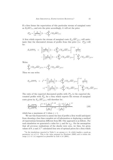
are irrational expectations rational? David Demery Nigel W. Duck1 ...

Are Irrational Expectations Rational? 15If a firm forms the expectation of this particular stream of marginal costsas E 2 MC t+i and sets the price accordingly, it will set the price:· ¸Pj,2 ∗ φ∞X= [1 − z] z i E 2 MCφ − 1g t+i0A firm which expects the stream of marginal costs E g j,1 MC j,t+i will anticipatethat the discounted stream of profits from this price (i.e. Pj,2 ∗ )willbe:"· ¸#φ∞X1−φE 1 DPF 2 =[1 − z] z i E j,2 MCφ − 1g 1t+i .1 − z0"· ¸#φ∞X−φ− [1 − z] z i E j,2 MCφ − 1g X ∞j,t+i z i E g j,1 MC j,t+iWrite:∞Xz i E g ∞Xj,2 MC j,t+i = ζ z i E j,1 MC g j,t+i00Then we can write:00"· ¸ φE j,1 DPF 2 = ζ 1−φ [1 − z]φ − 1"· φ−ζ −φ φ − 1¸[1 − z]#∞X1−φx i E g 1j,1 MC j,t+i .1 − z0#∞X−φz i E g X ∞j,1 MC j,t+i z i E j,1 MC g j,t+i00The ratio of the expected discounted profits with Pj,2 ∗ to the expected discountedprofits with Pj,1 ∗ for a firm which expects the stream of marginalcosts given by E g j,1 MC j,t+i will therefore be:³E j,1 DPF 2= ζ(1−φ) φ´(1−φ) ³−φ´³φ−1 −φ´−φζφ−1³E j,1 DPF 1 φ´(1−φ) ³ (10)φ−1 − φ´−φφ−1which has a maximum of 1 when ζ =1.We use this framework to assess the loss of profits a firm would anticipatefrom choosing a less than complete set of information or deploying a methodof expectations formation different from RE. Our approach is as follows. Foreach simulation we generated a value for ε t and for u j,t . On the assumptionthat all previous realizations of the shocks were zero, we then, for givenvalues of θ, φ and β, 11 calculated four sets of optimal prices for a firm which11 In the simulations reported in Table 5, we assume φ =6, which implies a mark-upparameter (ϕ) of 1.2. This is the value assumed by Sbordone (2002) and is within therange (1.1 to 1.4) suggested as plausible by Galí et al (2001).