An estimated dynamic stochastic general equilibrium model of the ...

More documents

Recommendations

Info

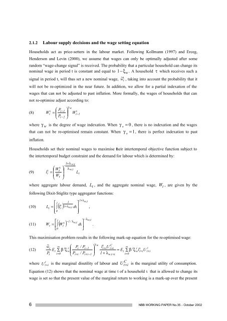
2.1.2 Labour supply decisions and the wage setting equationHouseholds act as price-setters in the labour market. Following Kollmann (1997) and Erceg,Henderson and Levin (2000), we assume that wages can only be optimally adjusted after somerandom “wage-change signal” is received. The probability that a particular household can change itsnominal wage in period t is constant and equal to 1 −ξ w . A household τ which receives such aιsignal in period t, will thus set a new nominal wage, w ~ t , taking into account the probability that itwill not be re-optimized in the near future. In addition, we allow for a partial indexation of thewages that can not be adjusted to past inflation. More formally, the wages of households that cannot re-optimise adjust according to:(8)Wιt⎛ P=⎜⎝ Pt−1t−2⎞⎟ ⎠γ wWιt−1where γ w is the degree of wage indexation. When γw= 0 , there is no indexation and the wagesthat can not be re-optimised remain constant. When γ = 1, there is perfect indexation to pastinflation.Households set their nominal wages to maximise their intertemporal objective function subject tothe intertemporal budget constraint and the demand for labour which is determined by:1+λ w t,−⎛ ιW ⎞ λι t w,t(9) l ⎟t = ⎜Lt⎜ Wt⎟⎝ ⎠where aggregate labour demand,following Dixit-Stiglitz type aggregator functions:⎡1ι(10) L ⎢∫( l )⎡1ι(11) W ∫ ( W )tt1+λw,t1 ⎤= 1+λt w,t dι⎥,⎢⎣0 ⎥⎦−λw,t−1 / λw,t⎤= ⎢ t dι⎥.⎣0⎦L t , and the aggregate nominal wage,wW t , are given by theThis maximisation problem results in the following mark-up equation for the re-optimised wage:∞w Cw ~γ ι⎛(12) ∑⎟ ⎞∞t i i P⎜t / Pt−1l t + i U t + iiEtβ ξ w= Et∑ β ξPti= 0 ⎝ Pt+ i / Pt+ i−1⎠ 1 + λw,t+ i i=0wherelU t+ iis the marginal disutility of labour andi ιwlt+iUlt+iCU t+i is the marginal utility of consumption.Equation (12) shows that the nominal wage at time t of a household ι that is allowed to change itswage is set so that the present value of the marginal return to working is a mark-up over the present6 NBB WORKING PAPER No.35 - October 2002
value of marginal cost (the subjective cost of working). 10 When wages are perfectly flexible( ξ w = 0 ), the real wage will be a mark-up (equal to 1+ λ w, t ) over the current ratio of the marginaldisutility of labour and the marginal utility of an additional unit of consumption. We assume thatwshocks to the wage mark-up, λ w, t = λw+ ηt, are IID-Normal around a constant.Given equation (11), the law of motion of the aggregate wage index is given by:γ−1/λww t,⎛1 /P ⎞− λt 11/t w t 1ww ~ λξ⎜ ⎛ − ⎞ ⎟−⎜ −⎜ξ tP⎟⎟t−2(13) ( W )w,t= W+ (1 − )( )w, t2.1.3 Investment and capital accumulation⎝⎝⎠⎠Finally, households own the capital stock, a homogenous factor of production, which they rent outkto the firm-producers of intermediate goods at a given rental rate of r t . They can increase thesupply of rental services from capital either by investing in additional capital ( I t ), which takes oneperiod to be installed or by changing the utilisation rate of already installed capital ( z t ). Bothactions are costly in terms of foregone consumption (see the intertemporal budget constraint (4) and(5)). 11Households choose the capital stock, investment and the utilisation rate in order to maximise theirintertemporal objective function subject to the intertemporal budget constraint and the capitalaccumulation equation which is given by:I(14) Kt= Kt−1 [ 1−] + [ 1−S( εtI t / I t −1)] I tτ ,where I t is gross investment, τ is the depreciation rate and the adjustment cost function S (.) is apositive function of changes in investment. 12 S (.) equals zero in steady state with a constantinvestment level. In addition, we assume that the first derivative also equals zero aroundequilibrium, so that the adjustment costs will only depend on the second-order derivative as in CEE(2001). We also introduce a shock to the investment cost function, which is assumed to follow aI I Ifirst-order autoregressive process with an IID-Normal error term: ε t = ρIεt−1 + ηt. 1310111213Standard RBC models typically assume an infinite supply elasticity of labour in order to obtain realistic business cycleproperties for the behaviour of real wages and employment. An infinite supply elasticity limits the increase inmarginal costs and prices following an expansion of output in a model with sticky prices, which helps to generate realpersistence of monetary shocks. The introduction of nominal-wage rigidity in this model makes the simulationoutcomes less dependent on this assumption, as wages and the marginal cost become less sensitive to output shocks, atleast over the short term.This specification of the costs is preferable above a specification with costs in terms of a higher depreciation rate (seeKing and Rebelo, 2000; or Greenwood, Hercowitz, and Huffman, 1988; Dejong, Ingram and Whiteman, 2000)because the costs are expressed in terms of consumption goods and not in terms of capital goods. This formulationlimits further the increase in marginal cost of an output expansion (See CEE, 2001).See CEE (2001).See, Keen (2001) for a recent DSGE model with sticky prices in which one of the shocks comes from changes in costsof adjusting investment.NBB WORKING PAPER No. 35 - October 2002 7
Page 3 and 4: AbstractThis paper develops and est
Page 5 and 6: TABLE OF CONTENTS:1. INTRODUCTION..
Page 7 and 8: 1. IntroductionIn this paper we pre
Page 9 and 10: shock leads to a gradual increase i
Page 14 and 15: The first-order conditions result i
Page 16 and 17: jt⎛⎜ p− MCtt )⎜⎝Ptp,t(24)
Page 18 and 19: where β = 1/(1−τ+ r k ) . The c
Page 20: price and wages in the absence of t
Page 23 and 24: whereÊ t denotes the number of peo
Page 25 and 26: curve for a normal distribution wit
Page 27 and 28: where p(θ A ) is the prior density
Page 29 and 30: 3.3.2 Comparison of empirical and m
Page 31 and 32: the effects on marginal cost and in
Page 33 and 34: 4.3 Historical decompositionGraphs
Page 35 and 36: very much in response to the variou
Page 37 and 38: estimate of potential output should
Page 39 and 40: Table 1: Parameter estimatesPrior d
Page 41 and 42: Table 3: Variance decompositionC I
Page 43 and 44: 300020001000persistence productivit
Page 46 and 47: Graph 3: Productivity shock (1)0.50
Page 48 and 49: Graph 5: Wage mark-up shock0.050yc0
Page 50 and 51: Graph 7: Preference shock1.210.8yc0
Page 52 and 53: Graph 9: Equity premium shock0.30.2
Page 54 and 55: Graph 11: Monetary policy shock0-0.
Page 56 and 57: Graph 13: Inflation decomposition -
Page 58 and 59: Graph 16: Labour supply shock: flex
Page 60 and 61: Graph 18: Investment shock: flexibl
Page 62 and 63:
Graph 20: Natural Output Gap105Natu
Page 64 and 65:
ReferencesAbel A.D. (1990), “Asse
Page 66 and 67:
Geweke J. (1999), “Computational
Page 68 and 69:
NATIONAL BANK OF BELGIUM - WORKING
Page 70 and 71:
24. "The impact of uncertainty on i
show all

An estimated dynamic stochastic general equilibrium model of the ...

Create successful ePaper yourself

Delete template?

Save as template?