An estimated dynamic stochastic general equilibrium model of the ...

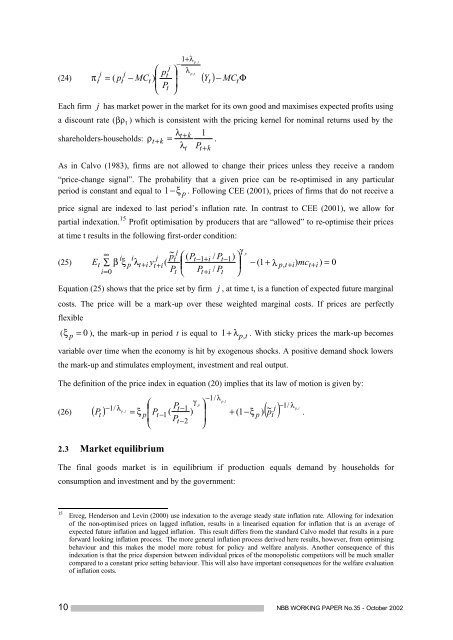
jt⎛⎜ p− MCtt )⎜⎝Ptp,t(24) ( ) − Φπ= ( pjtj⎞⎟⎟⎠1+λ−λp , tYtMCEach firm j has market power in the market for its own good and maximises expected profits usinga discount rate ( βρ t ) which is consistent with the pricing kernel for nominal returns used by theλshareholders-households:t+k 1ρ t+ k =.λtP t + kAs in Calvo (1983), firms are not allowed to change their prices unless they receive a random“price-change signal”. The probability that a given price can be re-optimised in any particularperiod is constant and equal to 1 −ξ p . Following CEE (2001), prices of firms that do not receive aprice signal are indexed to last period’s inflation rate. In contrast to CEE (2001), we allow forpartial indexation. 15 Profit optimisation by producers that are “allowed” to re-optimise their pricesat time t results in the following first-order condition:∞~ jγpi i j p ( / )(25) (t ⎛ P 1 1 ⎞⎜t−+ i PEt−t ∑ β ξ p λt+ i y t + i⎟ − (1 + λ p,t+i)mct+i)= 0i=0Pt⎝ Pt+ i / Pt⎠Equation (25) shows that the price set by firm j , at time t, is a function of expected future marginalcosts. The price will be a mark-up over these weighted marginal costs. If prices are perfectlyflexible( ξ p = 0 ), the mark-up in period t is equal to 1+ λ p, t . With sticky prices the mark-up becomesvariable over time when the economy is hit by exogenous shocks. A positive demand shock lowersthe mark-up and stimulates employment, investment and real output.The definition of the price index in equation (20) implies that its law of motion is given by:−Pt−1/λ⎛γP ⎞j −1/λ= ξ ⎜p Pt1 ( ) ⎟−+ (1 −ξp ) pt.⎜ Pt−2⎟⎝⎠p,tp1 / λt−1~p tt(26) ( ) ( ) p,,2.3 Market equilibriumThe final goods market is in equilibrium if production equals demand by households forconsumption and investment and by the government:t15Erceg, Henderson and Levin (2000) use indexation to the average steady state inflation rate. Allowing for indexationof the non-optimised prices on lagged inflation, results in a linearised equation for inflation that is an average ofexpected future inflation and lagged inflation. This result differs from the standard Calvo model that results in a pureforward looking inflation process. The more general inflation process derived here results, however, from optimisingbehaviour and this makes the model more robust for policy and welfare analysis. Another consequence of thisindexation is that the price dispersion between individual prices of the monopolistic competitors will be much smallercompared to a constant price setting behaviour. This will also have important consequences for the welfare evaluationof inflation costs.10 NBB WORKING PAPER No.35 - October 2002