An estimated dynamic stochastic general equilibrium model of the ...
An estimated dynamic stochastic general equilibrium model of the ...
An estimated dynamic stochastic general equilibrium model of the ...
Create successful ePaper yourself
Turn your PDF publications into a flip-book with our unique Google optimized e-Paper software.
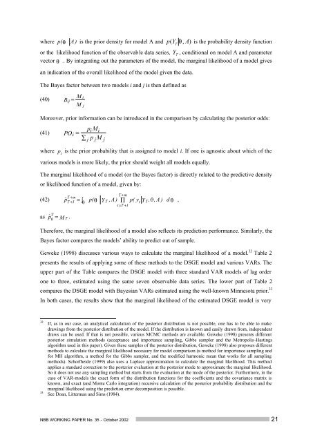
where p(θ A ) is <strong>the</strong> prior density for <strong>model</strong> A and p( Y Tθ , A)is <strong>the</strong> probability density functionor <strong>the</strong> likelihood function <strong>of</strong> <strong>the</strong> observable data series, YT, conditional on <strong>model</strong> A and parametervector θ . By integrating out <strong>the</strong> parameters <strong>of</strong> <strong>the</strong> <strong>model</strong>, <strong>the</strong> marginal likelihood <strong>of</strong> a <strong>model</strong> givesan indication <strong>of</strong> <strong>the</strong> overall likelihood <strong>of</strong> <strong>the</strong> <strong>model</strong> given <strong>the</strong> data.The Bayes factor between two <strong>model</strong>s i and j is <strong>the</strong>n defined as(40)Bij =MMijMoreover, prior information can be introduced in <strong>the</strong> comparison by calculating <strong>the</strong> posterior odds:p(41) = iMiPO i∑ j p jMjwhere p iis <strong>the</strong> prior probability that is assigned to <strong>model</strong> i. If one is agnostic about which <strong>of</strong> <strong>the</strong>various <strong>model</strong>s is more likely, <strong>the</strong> prior should weight all <strong>model</strong>s equally.The marginal likelihood <strong>of</strong> a <strong>model</strong> (or <strong>the</strong> Bayes factor) is directly related to <strong>the</strong> predictive densityor likelihood function <strong>of</strong> a <strong>model</strong>, given by:T+mT + m+,θt=T + 1(42) pˆT 1= ∫ p( θ YT, A ) ∏ p( ytYT,ϑ,A ) d θasTpˆ0 = M T .Therefore, <strong>the</strong> marginal likelihood <strong>of</strong> a <strong>model</strong> also reflects its prediction performance. Similarly, <strong>the</strong>Bayes factor compares <strong>the</strong> <strong>model</strong>s’ ability to predict out <strong>of</strong> sample.Geweke (1998) discusses various ways to calculate <strong>the</strong> marginal likelihood <strong>of</strong> a <strong>model</strong>. 32 Table 2presents <strong>the</strong> results <strong>of</strong> applying some <strong>of</strong> <strong>the</strong>se methods to <strong>the</strong> DSGE <strong>model</strong> and various VARs. Theupper part <strong>of</strong> <strong>the</strong> Table compares <strong>the</strong> DSGE <strong>model</strong> with three standard VAR <strong>model</strong>s <strong>of</strong> lag orderone to three, <strong>estimated</strong> using <strong>the</strong> same seven observable data series. The lower part <strong>of</strong> Table 2compares <strong>the</strong> DSGE <strong>model</strong> with Bayesian VARs <strong>estimated</strong> using <strong>the</strong> well-known Minnesota prior. 33In both cases, <strong>the</strong> results show that <strong>the</strong> marginal likelihood <strong>of</strong> <strong>the</strong> <strong>estimated</strong> DSGE <strong>model</strong> is very3233If, as in our case, an analytical calculation <strong>of</strong> <strong>the</strong> posterior distribution is not possible, one has to be able to makedrawings from <strong>the</strong> posterior distribution <strong>of</strong> <strong>the</strong> <strong>model</strong>. If <strong>the</strong> distribution is known and easily drawn from, independentdraws can be used. If that is not possible, various MCMC methods are available. Geweke (1998) presents differentposterior simulation methods (acceptance and importance sampling, Gibbs sampler and <strong>the</strong> Metropolis-Hastingsalgorithm used in this paper). Given <strong>the</strong>se samples <strong>of</strong> <strong>the</strong> posterior distribution, Geweke (1998) also proposes differentmethods to calculate <strong>the</strong> marginal likelihood necessary for <strong>model</strong> comparison (a method for importance sampling andfor MH algorithm, a method for <strong>the</strong> Gibbs sampler, and <strong>the</strong> modified harmonic mean that works for all samplingmethods). Schorfheide (1999) also uses a Laplace approximation to calculate <strong>the</strong> marginal likelihood. This methodapplies a standard correction to <strong>the</strong> posterior evaluation at <strong>the</strong> posterior mode to approximate <strong>the</strong> marginal likelihood.So it does not use any sampling method but starts from <strong>the</strong> evaluation at <strong>the</strong> mode <strong>of</strong> <strong>the</strong> posterior. Fur<strong>the</strong>rmore, in <strong>the</strong>case <strong>of</strong> VAR-<strong>model</strong>s <strong>the</strong> exact form <strong>of</strong> <strong>the</strong> distribution functions for <strong>the</strong> coefficients and <strong>the</strong> covariance matrix isknown, and exact (and Monte Carlo integration) recursive calculation <strong>of</strong> <strong>the</strong> posterior probability distribution and <strong>the</strong>marginal likelihood using <strong>the</strong> prediction error decomposition is possible.See Doan, Litterman and Sims (1984).NBB WORKING PAPER No. 35 - October 2002 21


