Morphology of Experimental and Simulated Turing Patterns

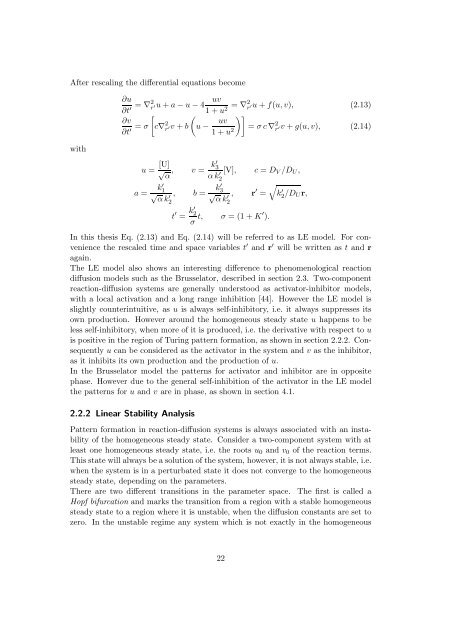
After rescaling the differential equations becomewith∂u∂t ′ = ∇ 2 uvr ′u + a − u − 41 + u 2 = ∇2 r ′u + f(u,v), (2.13)(∂v∂t ′ = σ[c∇ 2 r ′v + b u −uv )]1 + u 2 = σ c ∇ 2 r ′v + g(u,v), (2.14)u = √ [U] , v = k′ 3α αk 2′ [V], c = D V /D U ,a = k′ 1√ αk′, b = k′ 3√2 α k′, r ′ =2t ′ = k′ 2σ t, σ = (1 + K′ ).√k ′ 2 /D Ur,In this thesis Eq. (2.13) and Eq. (2.14) will be referred to as LE model. For conveniencethe rescaled time and space variables t ′ and r ′ will be written as t and ragain.The LE model also shows an interesting difference to phenomenological reactiondiffusion models such as the Brusselator, described in section 2.3. Two-componentreaction-diffusion systems are generally understood as activator-inhibitor models,with a local activation and a long range inhibition [44]. However the LE model isslightly counterintuitive, as u is always self-inhibitory, i.e. it always suppresses itsown production. However around the homogeneous steady state u happens to beless self-inhibitory, when more of it is produced, i.e. the derivative with respect to uis positive in the region of Turing pattern formation, as shown in section 2.2.2. Consequentlyu can be considered as the activator in the system and v as the inhibitor,as it inhibits its own production and the production of u.In the Brusselator model the patterns for activator and inhibitor are in oppositephase. However due to the general self-inhibition of the activator in the LE modelthe patterns for u and v are in phase, as shown in section 4.1.2.2.2 Linear Stability AnalysisPattern formation in reaction-diffusion systems is always associated with an instabilityof the homogeneous steady state. Consider a two-component system with atleast one homogeneous steady state, i.e. the roots u 0 and v 0 of the reaction terms.This state will always be a solution of the system, however, it is not always stable, i.e.when the system is in a perturbated state it does not converge to the homogeneoussteady state, depending on the parameters.There are two different transitions in the parameter space. The first is called aHopf bifurcation and marks the transition from a region with a stable homogeneoussteady state to a region where it is unstable, when the diffusion constants are set tozero. In the unstable regime any system which is not exactly in the homogeneous22