Morphology of Experimental and Simulated Turing Patterns

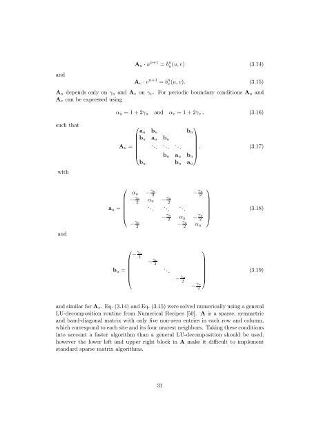
andA u · u n+1 = b n u (u,v) (3.14)A v · v n+1 = b n v(u,v). (3.15)A u depends only on γ u and A v on γ v . For periodic boundary conditions A u andA v can be expressed usingα u = 1 + 2γ u and α v = 1 + 2γ v , (3.16)such thatwith⎛⎞a u b u b ub u a u b uA u =. .. . .. . ... (3.17)⎜⎟⎝ b u a u b u⎠b u b u a uand⎛a u =⎜⎝⎞α u − γu 2− γu 2− γu 2α u − γu 2. .. . .. . ..⎟− γu 2α u − γu ⎠2− γu 2− γu 2α u(3.18)⎛b u =⎜⎝− γu 2− γu 2. ..− γu 2⎞⎟⎠(3.19)− γu 2and similar for A v . Eq. (3.14) and Eq. (3.15) were solved numerically using a generalLU-decomposition routine from Numerical Recipes [50]. A is a sparse, symmetricand band-diagonal matrix with only five non-zero entries in each row and column,which correspond to each site and its four nearest neighbors. Taking these conditionsinto account a faster algorithm than a general LU-decomposition should be used,however the lower left and upper right block in A make it difficult to implementstandard sparse matrix algorithms.31