Morphology of Experimental and Simulated Turing Patterns

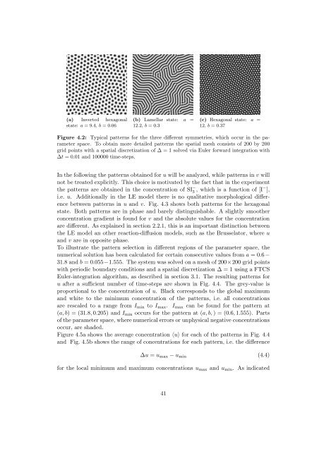
(a) Inverted hexagonalstate: a = 9.4, b = 0.06(b) Lamellar state: a =12.2, b = 0.3(c) Hexagonal state: a =12, b = 0.37Figure 4.2: Typical patterns for the three different symmetries, which occur in the parameterspace. To obtain more detailed patterns the spatial mesh consists of 200 by 200grid points with a spatial discretization of ∆ = 1 solved via Euler forward integration with∆t = 0.01 and 100000 time-steps.In the following the patterns obtained for u will be analyzed, while patterns in v willnot be treated explicitly. This choice is motivated by the fact that in the experimentthe patterns are obtained in the concentration of SI − 3 , which is a function of [I− ],i.e. u. Additionally in the LE model there is no qualitative morphological differencebetween patterns in u and v. Fig. 4.3 shows both patterns for the hexagonalstate. Both patterns are in phase and barely distinguishable. A slightly smootherconcentration gradient is found for v and the absolute values for the concentrationare different. As explained in section 2.2.1, this is an important distinction betweenthe LE model an other reaction-diffusion models, such as the Brusselator, where uand v are in opposite phase.To illustrate the pattern selection in different regions of the parameter space, thenumerical solution has been calculated for certain consecutive values from a = 0.6 −31.8 and b = 0.055−1.555. The system was solved on a mesh of 200×200 grid pointswith periodic boundary conditions and a spatial discretization ∆ = 1 using a FTCSEuler-integration algorithm, as described in section 3.1. The resulting patterns foru after a sufficient number of time-steps are shown in Fig. 4.4. The grey-value isproportional to the concentration of u. Black corresponds to the global maximumand white to the minimum concentration of the patterns, i.e. all concentrationsare rescaled to a range from I min to I max . I max can be found for the pattern at(a,b) = (31.8,0.205) and I min occurs for the pattern at (a,b,) = (0.6,1.555). Partsof the parameter space, where numerical errors or unphysical negative concentrationsoccur, are shaded.Figure 4.5a shows the average concentration 〈u〉 for each of the patterns in Fig. 4.4and Fig. 4.5b shows the range of concentrations for each pattern, i.e. the difference∆u = u max − u min (4.4)for the local minimum and maximum concentrations u max and u min . As indicated41