Morphology of Experimental and Simulated Turing Patterns

More documents

Recommendations

Info

The ansatz from Eq. (3.24) yields[ξ − 1 − χ u1 + χ u− ∆t]f uδu 0 − ∆t1 + χ uf v1 + χ uδv 0 = 0 (3.34)and[ξ − 1 − χ v1 + χ v− ∆t]g vδv 0 − ∆t1 + χ vg u1 + χ vδu 0 = 0 (3.35)withχ u = 2γ u sin 2 k x∆2+ 2γ u sin 2 k y∆2(3.36)andχ v = 2γ v sin 2 k x∆2 + 2γ v sin 2 k y∆2 , (3.37)or as a matrix equation()fξ − β u −∆t v( )1+χ u δu0g−∆t u· = 0 (3.38)1+χ vξ − β v δv 0withβ u = 1 − χ u1 + χ u+ ∆tf u1 + χ uand β v = 1 − χ v1 + χ v+ ∆tg v1 + χ v. (3.39)Eq. (3.38) can only have nontrivial solutions if the determinant is zero. Consequentlywe get(ξ − β u ) (ξ − β v ) − (∆t) 2 f v g u = 0. (3.40)So the condition |ξ| < 1 has to be fullfilled for the solutionsξ ± = 1 [](β u + β v ) ±√(β u + β v ) 2 + 4(∆t) 2 f v g u . (3.41)2The stability depends on the time and spatial discretization ∆t, ∆ and the valuesof the linearized reaction terms f u ,f v and g u ,g v . However as 1 + χ u and 1 + χ vare always larger than one the stability is less dependent on ∆ for a suitable setof parameters than it is for the FTCS method. Common parameters used for thesemi-implicit method were ∆ = 1 and ∆t = 0.1, which ensures |ξ ± | < 1.34
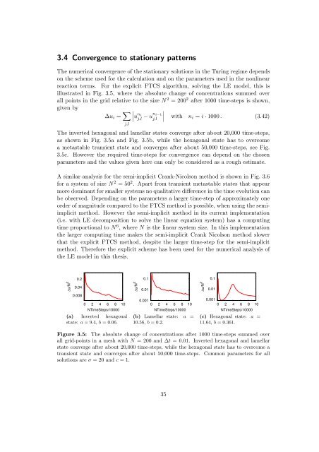
3.4 Convergence to stationary patternsThe numerical convergence of the stationary solutions in the Turing regime dependson the scheme used for the calculation and on the parameters used in the nonlinearreaction terms. For the explicit FTCS algorithm, solving the LE model, this isillustrated in Fig. 3.5, where the absolute change of concentrations summed overall points in the grid relative to the size N 2 = 200 2 after 1000 time-steps is shown,given by∆u i = ∑ ∣∣u n ij,l − un i−1j,l ∣ with n i = i · 1000. (3.42)j,lThe inverted hexagonal and lamellar states converge after about 20,000 time-steps,as shown in Fig. 3.5a and Fig. 3.5b, while the hexagonal state has to overcomea metastable transient state and converges after about 50,000 time-steps, see Fig.3.5c. However the required time-steps for convergence can depend on the chosenparameters and the values given here can only be considered as a rough estimate.A similar analysis for the semi-implicit Crank-Nicolson method is shown in Fig. 3.6for a system of size N 2 = 50 2 . Apart from transient metastable states that appearmore dominant for smaller systems no qualitative difference in the time evolution canbe observed. Depending on the parameters a larger time-step of approximately oneorder of magnitude compared to the FTCS method is possible, when using the semiimplicitmethod. However the semi-implicit method in its current implementation(i.e. with LE decomposition to solve the linear equation system) has a computingtime proportional to N 6 , where N is the linear system size. In this implementationthe larger computing time makes the semi-implicit Crank Nicolson method slowerthat the explicit FTCS method, despite the larger time-step for the semi-implicitmethod. Therefore the explicit scheme has been used for the numerical analysis ofthe LE model in this thesis.∆u/N 20.20.040.0080 2 4 6 8 10NTimeSteps/10000(a) Inverted hexagonalstate: a = 9.4, b = 0.06.∆u/N 20.10.010.0010 2 4 6 8 10NTimeSteps/10000(b) Lamellar state: a =10.56, b = 0.2.∆u/N 20.10.010.0010 2 4 6 8 10NTimeSteps/10000(c) Hexagonal state: a =11.64, b = 0.361.Figure 3.5: The absolute change of concentrations after 1000 time-steps summed overall grid-points in a mesh with N = 200 and ∆t = 0.01. Inverted hexagonal and lamellarstate converge after about 20,000 time-steps, while the hexagonal state has to overcome atransient state and converges after about 50,000 time-steps. Common parameters for allsolutions are σ = 20 and c = 1.35
Page 5: AbstractTuring patterns formed in t
Page 10: 5.5 Minkowski-maps of patterns in t
Page 13 and 14: of the experimental quasi-2D patter
Page 15: (a) “Bacteria” in a reactiondif
Page 18 and 19: Figure 2.1: First evidence for Turi
Page 20 and 21: 2.2 Lengyel-Epstein (LE) model for
Page 22 and 23: After rescaling the differential eq
Page 24 and 25: A full derivation is given in Ref.
Page 27 and 28: Chapter 3Numerical solution of 2Dre
Page 29 and 30: The advantage of the FTCS method is
Page 31 and 32: andA u · u n+1 = b n u (u,v) (3.14
Page 33: withχ u = 2γ u sin 2 k x∆2+ 2γ
Page 37 and 38: 3.5 Discretization of stochastic pa
Page 39 and 40: Chapter 4Patterns in the Lengyel-Ep
Page 41 and 42: (a) Inverted hexagonalstate: a = 9.
Page 43 and 44: Figure 4.4: Overview of pattern for
Page 45 and 46: 1.61.41.21b0.80.60.40.205 10 15 20
Page 47 and 48: 1.61.41.21b0.80.60.40.205 10 15 20
Page 49: Figure 4.10: The concentration prof
Page 52 and 53: (a) ρ = 0.22, V = 0.77, S =0.15,
Page 54 and 55: Figure 5.2: Illustration for the ma
Page 56 and 57: perimeter S(ρ) and the Euler chara
Page 58 and 59: (a) Experimental hexagonalpattern.
Page 60 and 61: 5.3 Minkowski functionals of simula
Page 62 and 63: (a) Numerical hexagonalpattern, b =
Page 64 and 65: (a) Experimental hexagonalpattern(b
Page 66 and 67: 5.4 Local Minkowski functionals of
Page 68 and 69: P V3210-1-2-1 -0.5 0 0.5 1ρP S2.42
Page 70 and 71: (a) Experimental hexagonalpattern(b
Page 72 and 73: 5.5 Minkowski-maps of patterns in t
Page 74 and 75: V(ρ)10.80.60.40.200 0.2 0.4 0.6 0.
Page 76 and 77: (a) Experimental hexagonalpattern.
Page 78 and 79: 5.7 Minkowski functionals of patter
Page 81 and 82: Chapter 6Influence of additive nois
Page 83 and 84: ∆u/N 20.2∆u/N 20.1∆u/N 20.10.
Page 85 and 86:
(a) Experimental lamellae.(b) Numer
Page 87 and 88:
Chapter 7Statistical ensemble of su
Page 89 and 90:
HexagonalLamellar0.10.20.51.0amplit
Page 91 and 92:
Experimental patternSuperposed patt
Page 93 and 94:
In this model no dynamics are expli
Page 95 and 96:
Experimental patternSuperposed patt
Page 97 and 98:
7.3 Interacting pattern gasIn this
Page 99 and 100:
7.3.3 Numerical resultsIn this sect
Page 101 and 102:
60000040000050000040000035000030000
Page 103 and 104:
Chapter 8Summary and outlookA quant
Page 105 and 106:
•••••••••••
Page 107 and 108:
(a)(b)(c)(d)(e)(f)Figure 9.3: Patte
Page 109 and 110:
Appendix ADetails on experimental d
Page 111 and 112:
Bibliography[1] K. Agladze, E. Dulo
Page 113 and 114:
[28] I. Lengyel and J. A. Pojman. A
Page 115 and 116:
[54] B. Rudovics, E. Barillot, P. W
Page 117:
ErklärungHiermit bestätige ich, d
show all

Morphology of Experimental and Simulated Turing Patterns

You also want an ePaper? Increase the reach of your titles

Delete template?

Save as template?