Lab Proposal for Integrated Real-time and Control - DCS - UPC

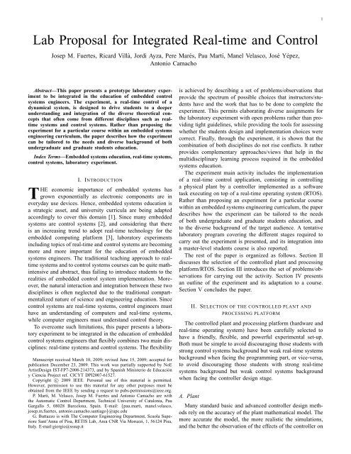
1Lab Proposal for Integrated Real-time and ControlJosep M. Fuertes, Ricard Villà, Jordi Ayza, Pere Marés, Pau Martí, Manel Velasco, José Yépez,Antonio CamachoAbstract—This paper presents a prototype laboratory experimentto be integrated in the education of embedded controlsystems engineers. The experiment, a real-time control of adynamical system, is designed to drive students to a deeperunderstanding and integration of the diverse theoretical conceptsthat often come from different disciplines such as realtimesystems and control systems. Rather than proposing theexperiment for a particular course within an embedded systemsengineering curriculum, the paper describes how the experimentcan be tailored to the needs and diverse background of bothundergraduate and graduate students education.Index Terms—Embedded systems education, real-time systems,control systems, laboratory experiment.I. INTRODUCTIONTHE economic importance of embedded systems hasgrown exponentially as electronic components are ineveryday use devices. Hence, embedded systems education isa strategic asset, and university curricula are being adaptedaccordingly to cover this domain [1]. Since many embeddedsystems are control systems [2], and considering that thereis an increasing trend to adopt real-time technology for theembedded computing platform [3], laboratory experimentsincluding topics of real-time and control systems are becomingmore and more important for the education of embeddedsystems engineers. The traditional teaching approach to realtimesystems and to control systems courses can be quite mathintensiveand abstract, thus failing to introduce students to therealities of embedded control system implementation. Moreover,the natural interaction and integration between these twodisciplines is often neglected due to the traditional compartmentalizednature of science and engineering education. Sincecontrol systems are real-time systems, control engineers musthave an understanding of computers and real-time systems,while computer engineers must understand control theory.To overcome such limitations, this paper presents a laboratoryexperiment to be integrated in the education of embeddedcontrol systems engineers that flexibly combines two main disciplines:real-time systems and control systems. The flexibilityManuscript received March 10, 2009; revised June 15, 2009; accepted forpublication December 23, 2009. This work was partially supported by NoEArtistDesign IST-FP7-2008-214373, and by Spanish Ministerio de Educacióny Ciencia Project ref. CICYT DPI2007-61527.Copyright c○ 2009 IEEE. Personal use of this material is permitted.However, permission to use this material for any other purposes must beobtained from the IEEE by sending a request to pubs-permissions@ieee.org.P. Martí, M. Velasco, Josep M. Fuertes and Antonio Camacho are withthe Automatic Control Department, Technical University of Catalonia, PauGargallo 5, 08028 Barcelona, Spain. E-mail: {pau.marti, manel.velasco,josep.m.fuertes, antonio.camacho.santiago}@upc.eduG. Buttazzo is with The Computer Engineering Department, Scuola SuperioreSant’Anna of Pisa, RETIS Lab, Area CNR Via Moruzzi, 1, 56124 Pisa,Italy. E-mail:giorgio@sssup.itis achieved by describing a set of problems/observations thatprovide the spectrum of possible choices that instructors/studentshave and the work that has to be done to complete theexperiment. This permits elaborating diverse assignments forthe laboratory experiment with open problems rather than providingtight guidelines, while providing the tools for assessingwhether the students design and implementation choices werecorrect. Finally, through the experiment, it is shown that thecombination of both disciplines do not rise conflicts. It ratherprovides complementary approaches/views that help in themultidisciplinary learning process required in the embeddedsystems education.The experiment main activity includes the implementationof a real-time control application, consisting in controllinga physical plant by a controller implemented as a softwaretask executing on top of a real-time operating system (RTOS).Rather than proposing an experiment for a particular coursewithin an embedded systems engineering curriculum, the paperdescribes how the experiment can be tailored to the needsof both undergraduate and graduate students education, andto the diverse background of the target audience. A tentativelaboratory program covering the different stages required tocarry out the experiment is presented, and its integration intoa master-level students course is also reported.The rest of the paper is organized as follows. Section IIdiscusses the selection of the controlled plant and processingplatform/RTOS. Section III introduces the set of problems/observationsfor carrying out the activity. Section IV presentsan outline of the experiment and its adaptation to a course.Section V concludes the paper.II. SELECTION OF THE CONTROLLED PLANT ANDPROCESSING PLATFORMThe controlled plant and processing platform (hardware andreal-time operating system) have been carefully selected tohave a friendly, flexible, and powerful experimental set-up.Both must be simple to avoid discouraging those students withstrong control systems background but weak real-time systemsbackground when facing the programming part, or vice-versa,to avoid discouraging those students with strong real-timesystems background but weak control systems backgroundwhen facing the controller design stage.A. PlantMany standard basic and advanced controller design methodsrely on the accuracy of the plant mathematical model. Themore accurate the model, the more realistic the simulations,and the better the observation of the effects of the controller on

2Fig. 1.Plant and control setup.(a) RCRC circuit(b) Control setupthe plant. Hence, the plant was selected among those for whichan accurate mathematical model could easily be derived.Plants such as an inverted pendulum or a direct currentmotor are the defacto plants for benchmark problems in controlengineering [4]. However, their modelling is not trivial andthe resulting model is often not accurate. This leads to a firstcontroller design that has to be adjusted by ”engineering experience”,thus requiring knowledge that is difficult to formalizeand transmit to the students. To avoid such a kind of drawbacks,a simple electronic circuit in the form of an RCRC(Figure 1a) was selected. The simplicity of its components andtheir simple and intuitive physical behavior have been the mainreasons for its selection. Note however that experiments usingother plants can be complementary to the approach presentedhere, e.g. [2], [5]–[7]. Indeed, Lim [6] also proposes electroniccircuits. However, they are slightly more sophisticated becausethey include operational amplifiers. Although richer dynamicscan be achieved, the intuitive behavior and thus the modelingof operational amplifiers is not straightforward.The selection of an electronic circuit as a plant has alsoanother important advantage: depending on the specific circuit,it can be directly plugged into a micro-controller without usingintermediate electronic components, as shown in Figure 1b,where the zoh box (zero order hold) represents the actuator andthe box above represents the sampler. That is, the transistortransistorlogic (TTL) level signals provided by the microcontrollercan be enough to carry out the control. Notethat this is not the case, for example, for many mechanicalsystems. Such a simplification in terms of hardware reducesthe modelling effort to study the plant and no models foractuators or sensors are required. Additional benefits of thesetypes of plants are that systems can be easily built, are cheap,have light weight, and can be easily transported and powered.The control objective would be to have the circuit outputvoltage V out (controlled variable) to track a reference signal orto settle to a constant value while meeting for example giventransient response specifications, which mandates to use trackingstructures. The control will be achieved by sampling V out ,executing the control algorithm and applying the calculatedcontrol signal to the circuit via varying the circuit input voltageV in (manipulated variable). Disturbances can be injected by avariable load voltage placed in parallel to the output voltage.B. Processing platformThe processing platform consists of the hardware platformand the real-time operating system. As hardware platform,a micro-controller based architecture was selected becauseembedded systems are typically implemented using this typeof hardware. Note, however, that too small micro-controllersmay not be powerful enough for running an RTOS, as discussedin [9]. Among the several possibilities available on themarket [10], it was decided to adopt the Flex board [11].The Flex board (in its full version) represents a good compromisebetween cost, processing power, and programmingflexibility. It was produced as a development board for buildingand testing real-time applications using standard componentsand open source software. The board includes a MicrochipdsPIC DSC micro-controller dsPIC33FJ256MC710, a socketfor the 100 pin Plug-In Module (PIM), an ICD2 (in-circuit debugger)programmer connector, a USB (Universal Serial Bus)connector for direct programming, power supply connectors,a set of leds for monitoring the board, an on-board MicrochipPIC18F2550 micro-controller for integrated programming, anda set of connectors for daughter boards piggybacking.The board has several key benefits that make it suitable tobe used for educational purposes. First has a robust electronicdesign, which is an important feature when it is employedby non skilled users. Second, it has a modular architecture,which allows users to easily develop home-made daughterboards using standards components. A set of daughter boardscan be added to the Flex board for easy development, suchas a multi-bus board equipped with CAN (Controller AreaNetwork), Ethernet, I2C (Inter-Integrated Circuit), and othercommunication protocols. On one hand, the availability ofCAN or Ethernet permits to build and experiment with networkedcontrol applications. On the other hand, the availablenetworks can be used for debugging purposes or for extractingdata from the board, which is a difficult task when dealing withembedded systems.As far as the real-time kernel is concerned, different possibilitieswere considered. First, many well-known real-timeoperating systems, such as real-time Linux [12], target processorsthat may be too powerful for embedded applications. Butmore important, their internal structure is often too complexfor those students with a low profile in (real-time) operatingsystems. Hence, it looks more desirable to work with smallreal-time kernels (see e.g. [13]–[18] for small real-time kernelstargeting small architectures) whose internals are accessible,easy to understand and modify, in order to tailor them to thespecific application needs. On the other hand, from a userpoint of view, programming and configuring the kernel (includingcreating tasks, assigning priorities/periods/deadlines,

3and setting the scheduling policy) should be friendly enoughto attract non-skilled programmers.From the considerations mentioned above, Erika Enterprisereal-time kernel [11] was selected. Erika provides full supportto the Flex board in terms of drivers, libraries, programmingfacilities, and sample applications. The kernel, available underthe General Public License and OSEK (Open Systems andtheir Interfaces for the Electronics in Motor Vehicles, [19])compliant, is a RTOS for small micro-controllers based on anAPI similar to those proposed by the OSEK consortium. Thekernel gives support for preemptive and non-preemptive multitasking,and implements several scheduling algorithms [20].The API provides support for tasks, events, alarms, resources,application modes, semaphores, and error handling. All thesefeatures permits to enforce real-time constraints to applicationtasks to show students the effects of sampling periods, delaysand jitter on control performance.The development environment for Erika Enterprise is basedon cross-compilation, avoiding typical students misconceptionswhen the development platform and the target sharethe same hardware. A tool, named RT-Druid [11] (based onEclipse [21]), can be used as a default development platformto program in C, with support from Microchip for the compilerand for the programming development kit. The latteris important because Microchip web-pages [22] are always agood place where to share experiments experiences and code:a good place for instructors and students to visit. RT-Druid implementsan OIL (OSEK Implementation Language) languagecompiler, which is able to generate the kernel configurationfrom an OIL specification. Apart from programming in C, theFlex board can also be programmed automatically using theScilab/Scicos [23] code generator (similar to what can be donewith MATLAB/Simulink [24] and its Real-Time Workshop, asused for example in [25] for rapid control prototyping). Thisis an important benefit for non-skilled C programmers.From an education point of view, it is also important to notethat there is the possibility to build a community around thisprocessing platform to create a repository of control softwarefor education. In fact, a set of application notes that describe aset of control experiments (inverted pendulum, ball and plate,etc.) developed with Erika on Flex can be found in [11].Finally, it must be stressed that the price of the Flex boardlies in the lower bound of evaluation board prices, and thatthe Erika kernel and the associated development tools areopen source, available for free, or available for free in studentedition format. Hence, it is an economically atractive option.III. EXAMPLE OF THE LAB EXPERIMENTThis section presents some of the activities in the form ofproblems and solutions (and observations) required to carryout the lab experience, which are later ordered in the workplan. The emphasis is in the control analysis and design part.A. Problem 1. Plant modellingIf q i represents the charge on capacitor C i , the differentialequations of the circuit, in terms of the currents ˙q i at each R i ,are given by˙q 1 R 1 +(q 1 −q 2 ) 1 C 1= V in˙q 2 R 2 +(q 2 −q 1 ) 1 1+q 2C 1 C 2= 0 (1)q 21C 2= V out ,For example, using state-space formalism, a state-spaceform is given byẋ(t) =y(t) =[]0 1−1x(t)R 1R 2C 1C 2−[ ]R1C1+R2C2+R1C2R 1R 2C 1C 20(2)+ 1 u(t)[ R 1R] 2C 1C 21 0 x(t)where u(t) is the control signal, y(t) is the plant output, andx(t) = [ x 1 x 2 ] is the state vector, where x 1 correspondsto the output voltage V out , and x 2 is ˙q 2 /C 2 .Observation 1: The modelling of the plant could have beenalso done in terms of a transfer function (see [26] for theanalysis). Even obtaining the differential equations is a goodexercise. Adopting the state space formalism may add anotherbenefit if using model (2). Since only the output voltagex 1 canbe physically measured, the control algorithm requires the useof observers for predicting x 2 . This opens the door to experimentwith several types of observers and the implementationof the controller has to include them. Also, the selection of thestate variables is arbitrary, and therefore, students have to takedesign decisions. For example, the voltages in both capacitorscould also have been chosen as a state variables. In any case,if possible, it is interesting to chose the state variables in sucha way that the controlled variable is directly available throughthe output matrix in order to minimize computations in themicro-controller.B. Problem 2. Electronic componentsThe selection of the electronic components is very importantfor several reasons. The output impedance must be lowenough to properly connect the circuit to the analog-to-digitalconverter (ADC) or to some external instrumentation, suchas an oscilloscope. For example, given the initial componentsR 1 = R 2 = 1 KΩ andC 1 = C 2 = 33µF, a manageable circuitimpedance is obtained. With these components, the state spacemodel becomes[ ] [ ]0 1 0ẋ(t) =x(t)+ u(t)−976.56 −93.75 976.56y(t) = [ 1 0 ] x(t).(3)Observation 2: Students can be given other values. Forexample, with R 1 = R 2 = 330 KΩ and C 1 = C 2 = 100ηF, it is easy to see that the equivalent output impedance istoo high for the ADC. To derive such a conclusion, studentshave to consult the dsPIC data sheet.

5CPU mySystem {OS myOs {EE_OPT = "DEBUG";CPU_DATA = PIC30 { APP_SRC = "code.c";MULTI_STACK = FALSE;ICD2 = TRUE;};MCU_DATA = PIC30 { MODEL = PIC33FJ256MC710;};BOARD_DATA = EE_FLEX { USELEDS = TRUE;};KERNEL_TYPE = EDF { NESTED_IRQ = TRUE;TICK_TIME = "25ns";};};TASK myTask {REL_DEADLINE = "10ms";PRIORITY = 1;STACK = SHARED;SCHEDULE = FULL;};COUNTER myCounter;ALARM myAlarm {COUNTER = "myCounter";ACTION = ACTIVATETASK {TASK = "myTask";};};};int main(void){T1_program();EE_time_init(); // EDF initializationADC_init(); // ADC1 configurationPWM_config(); // PWM1 configurationSetRelAlarm(myAlarm, 1, 10);for (;;){ // generationDelay(100000);reference = 2.5;Delay(100000);reference = 1;}return 0;}Fig. 4.Main code// reference signalFig. 3.Kernel configuration fileObservation 6: As before, simulations can be done usingdifferent methods.G. Problem 7. Controller design: observersFor the simulation, the two state variables are available.However, in the real experiment, an observer must be included.For simplicity in coding the control task, a reduced observercan been chosen for observing the second state variablex 2 . Forexample, the observer discrete gain is K r = −37.81 or K r =−13.42 for the fast and overshoot controller if the observercontinuous closed loop pole are located at p ob = −50.Observation 7: Students can design and evaluate by simulationdifferent types of observers (reduced, complete, etc.)with different dynamics. That is, they can also evaluate theeffect of different locations for the observer poles. Froman implementation point of view, students can also assessthe effect that splitting the control algorithm into two parts(calculate control signal and update state) has on input-outputdelays and schedulability [28].H. Problem 8. Implementation: kernel configuration and controlalgorithmThe first implementation involves coding the controller ina periodic task that will execute in isolation on top of Erika.The main pseudo-codes are illustrated in Figures 3, 4 and 5.Figure 3 is the conf.oil file that specifies the kernel configurationwith EDF (Earliest Deadline First, [27]) schedulingalgorithm and a periodic task that will be used to implement,for instance, the fast controller. The basics of the main codeare illustrated in Figure 4. First, the timer T1 is initialized and,together with SetRelAlarm, will produce the periodic activationof the control task every 10 ms (the processor speed wasconfigured at 40 MIPS - Million Instructions Per Second).Figure 5 shows the control task code including the observerand the tracking structure.Observation 8: Carrying out the kernel configuration andprogramming the controller could be taught following anordered sequence of steps, such as: 1) introduction to kernelconfiguration, 2) introduction to periodic tasks, 3) introductionto input/output operations (PWM, ADC).TASK(myTask){x_1 = read_adc()r = reference;x_2 = observer(Kr,x1,r,x_1old,x_2old);u = r*NU + K_1*(r*NX_1 - x_1) + k_2*(r*NX_2 - x_2);write_pwm(u);x_1old = x_1;x_2old = x_2;}Fig. 5.Control task codeI. Problem 9. Implementation: setup and monitoring detailsFigure 6a shows the experimental setup that includes anoscilloscope (for displaying the circuit output voltage) toshow the open loop response (Figure 6b) and the closed loopresponses (Figures 7a and b) achieved by each controllerexecuting in isolation. The oscilloscope screen-shots confirmthat the implementation achieves the control goal: the systemoutput performs the desired fast tracking or achieves thespecified overshoot.Observation 9: An oscilloscope has been used to monitorboth the responses. It can also be of interest to monitor whetherthe control task executes when specified. Another option couldbe to use the Multibus board to send the data of interest viaEthernet or any other available communication protocol. Thiswould pose interesting challenges in terms of the real-timesystem such as non-invasive debugging.J. Problem 10. Multitasking: simulationA second implementation is introduced to illustrate moreadvanced concepts. In the previous implementation a controltask was executing in isolation. However, in many hightechsystems, the processor is used not only for the controlcomputation, but also for interrupt handling, error management,monitoring, etc. And it is known that in a multitaskingreal-time control systems, jitters, i.e. timing interferences oncontrol tasks due to the concurrent execution of other tasks,deteriorate control loops performance [28]. The objective ofthis implementation is to observe these degrading effects andimplement corrective actions, e.g. [29]–[31].A starting point is to inject a new task in the kernel foreach control task. The new task, named noisy task, when tobe executed together with the fast controller, is given a period(and relative deadline) of 11 ms, and it is imposed an artificial

6(a) Fast closed loop response(a) Setup(b) Overshoot closed loop response(b) Open loop responseFig. 7.RCRC responses.Fig. 6.Experiment setup and monitoring.execution time of 9 ms. The noisy task that goes together withthe overshoot controller has a period and relative deadline of110 ms with 90 ms of execution time. The simulation of eachmultitasking system was done in the TrueTime simulator [32].Putting together each control task with the corresponding noisytask under EDF results in timing variability (jitter) for thecontrol task, as illustrated for the first multitasking system inthe schedule of Figure 8a. In this figure, the bottom curverepresents the execution of the fast controller task, whereasthe top curve represents the execution of the noisy task. Ineach graph, the low-level line denotes no-execution (that is,intervals in which the processor is idle), the middle level linedenotes a task ready to execute (i.e., waiting in the readyqueue), whereas the high-level line denotes a task in execution.Note that the control task has a measured execution time of0.12 ms, which is much less than the noisy task.Looking at the plant responses in Figures 8 b) and c), it canbe appreciated that the fast controller does not exhibit a controlperformance degradation, while the overshoot controller sufferssome degradation: overshoots are bigger, square amplitudediffers, transient response varies, etc. This fact indicates thatthe current control design for the fast controller is robustagainst jitters induced by scheduling, while the second oneis more fragile.Observation 10: Adopting an iterative simulation study,students can learn which parameters play an important rolewhen jitters appear. Are shorter sampling periods, or nonovershoottedresponses, a guarantee for having robust controldesigns? Which role do deadlines play in reducing jitters? Forfurther questions and solutions, see [33] and references therein.K. Problem 11. Multitasking: implementation and monitoringdetailsThe new implementation requires specifying the noisy taskby modifying the kernel oil file in terms of defining thenew task and the associated alarm. Also, the new task hasto be coded: forcing an artificial execution time is achievedby placing a delay into the code. The main code has to bemodified to configure the new alarm associated to the newtask.After the implementation, in the first multitasking system,it can be verified that scheduling conflicts (as illustrated inthe simulated schedule shown in Figure 8a) may occur, asillustrated in Figure 9a. In this sub-figure, the execution ofthe fast controller task sets an output pin to 0 and 1 ateach job start and finishing time. And the noisy task setsan output pin to 0 and 0.5 at each job start and finishingtime. In addition, similar responses for the fast and overshootcontroller are obtained (see sub-figures 9 b) and c)), showingthat the overshoot controller suffers degradation from jitters,while the fast controller shows the same response as it isexecuted in isolation. To illustrative purposes, Figure 10ashows the overshoot controller response when executing inisolation (dark curve) and when executing in the multitaskingsystem (grey curve).Observation 11: Undergraduate students may work the experimentup to this problem. It shows the importance of

732.521.510.50 0.5 1 1.5(a) Partial schedule(a) Partial schedule3.532.521.510.500 0.5 1 1.5 2(b) Faster multitasking closed loop response(b) Faster multitasking response3.532.521.510.500 0.5 1 1.5 2(c) Overshoot multitasking closed loopresponseFig. 8.Simulated multitasking RCRC responses and schedule.(c) Overshoot multitasking responseconcurrency and resource sharing with respect to controlperformance in a multitasking embedded control system.L. Problem 12: Multitasking: design for eliminating or minimizingthe jitter problemRecent research literature has faced the problems introducedby jitter and many solutions have been proposed. Here, thesolution proposed by Lozoya et al. [31] has been adopted.The basic idea is to synchronize the operations within eachcontrol loop at the actuation instants. In this way, the timeelapsed between consecutive actuation instants, named t k−1and t k , is exactly equal to the sampling period, h. Within thistime interval, the system state is sampled, named x s,k , andthe sampling time recorded, t s,k ∈ (t k−1 ,t k ). The differencebetween this time and the next actuation timeτ k = t k −t s,k (4)is used to estimate the state at the actuation instant asˆx k = Φ(τ k )x s,k +Γ(τ k )u k−1 (5)Fig. 9.Implemented multitasking RCRC responses and schedule.where Φ(t) = e At and Γ(t) = ∫ t0 eAs dsB, being A and Bthe system and input matrices in (3), and u k−1 the previouscontrol signal. Then, making use of ˆx k , the control commandis computed using the original control gain K asu k = Kˆx k . (6)The control command u k is held until the next actuationinstant. A control strategy using (4)-(6) relies on the timereference given by the actuation instants, if u k is applied to theplant by hardware interrupts, for example. In addition, samplesare not required to be periodic because τ k in (4) can vary ateach closed-loop operation.After implementing this strategy on the overshoot controllerin the multitasking system, Figure10 b) shows the result.Specifically, it shows the overshoot controller response whenexecuting in isolation (dark curve) and when executing in themultitasking system using the algorithm that eliminates jitters(grey curve).

8Fig. 10.(a) Overshoot controller with/withoutjitters(b) Overshoot controller eliminatingthe jitter problemOvershoot controller: degradation and solutionObservation 12: The problem presented above and its solutioncan be split into several tasks, like analysis and modellingof the new control algorithm, implementation of the controlalgorithm, etc. An interesting issue is how synchronized actuationinstants can be forced in the kernel. For example, asolution could be to use a periodic task for computing u k andanother periodic task for applying u k at the required time.Another solution could be to enforce synchronized executionsat the kernel level, using the EDF tick counter. Moreover,since different solutions to the jitter problem such as [29]or [30] could have also been applied, students more confidentor interested in specific fields can select the solution that bettermeets their preferences.IV. TENTATIVE WORK PLAN AND ITS APPLICATION TO ASPECIFIC COURSEThe previous section has detailed some of the steps requiredto successfully carry out the lab activity presented in this paper.This section summarizes them in order to propose a tentativework plan that is divided into several sessions, each one beinga two-hour lab.S1 - Introduction: Introduction to the activity, and simulationof the open-loop response after obtaining the statespaceform of the RCRC circuit from the circuit differentialequations (1) (consider random values for R and C). Here itis assumed that state-space notation is chosen.S2 - Problem specification (a): This session should beused to specify the problem in terms of the levels for thereference signal and for discrete controller design, whichincludes selecting the sampling period and closed loop polelocations, if pole placement is used. Other control approaches,like optimal control, could also be used.S3 - Problem specification (b): To complement the previoussession, observers should also be designed and simulated.The outcome of this session should be the complete simulationsetup.S4 - Basic implementation (a): Build the RCRC circuitand verify its dynamics in open-loop. Start the controller implementationin a periodic hard real-time task in the processingplatform.S5 - Basic implementation (b): Finish the controllerimplementation and test its correctness.S6 - Multitasking (a): Incorporate a noisy task in thesimulation setup to evaluate the effects of jitter. This stepwould require to use, for example, the TrueTime simulator.S7 - Multitasking (b): Incorporate the noisy task in theimplementation and validate the previous simulation results.S8 - Advanced implementation (a): If degradation in controlperformance is detected in the previous session, simulateadvanced control algorithms or adopt real-time techniques tosolve or reduce the jitter problem.S9 - Advanced implementation (b): Implement the previoussolutions and validate them.Note that the program timing, layout and the set of coveredtopics should be adapted to particular needs/background of thetarget audience or to the goals of the specific curriculum. Forexample, the proposed activity has been introduced as a partof the curriculum of the 2-year master degree on AutomaticControl and Industrial Electronics in the Engineering Schoolin Vilanova i la Geltrú (EPSEVG) of the Technical Universityof Catalonia (UPC) [34]. In particular, since 2007, theexperiment was tailored to become part of the laboratory forthe Control Engineering course, which covers continuous anddiscrete linear time invariant (LTI) control systems, as well asnon-linear control systems, all using state-space formalism.Sessions S1 to S5 were adopted for the laboratory of thediscrete LTI control systems part.The Control Engineering course can be followed by studentseither in the first semester of the first year or in the firstsemester of the second year. Students choosing the secondoption simultaneously attend a course on real-time systems.Therefore, within the same classroom, not all the students arefamiliar with real-time systems. To overcome this apparentdrawback, teams of three students were formed containing atleast a student with competence on real-time systems. Withinsuch heterogeneous teams in terms of skills and theoreticalbackground, it was observed that students took their responsibilitiesand team-work was significantly improved.As in every course edition, after finishing the discrete LTIcontrol systems part, a short and simple questionnaire is givento the students to let them evaluate several aspects of this partof the course. The question Do the laboratory activities permitto better understand the theoretical concepts? is the only onerelated to the laboratories. Looking at the students answers,and taking into account that before introducing the presentedexperiment the lab activities were focused on the simulation of

9an inverted pendulum, the percentage of students appreciatingthe practical part has increased significantly. Although thestandard course evaluation indicates this positive trend, amore complete evaluation tailored to the introduction of thisexperiment is required.V. CONCLUSIONSThis paper has presented a laboratory activity to be integratedin the education curriculum of embedded controlsystems engineers. The activity consists of a real-time controllerof a RCRC electronic circuit. The potential benefits,competences to be acquired, and expected learning outcomesfor students have been presented. The selection of the plant andprocessing platform has been discussed. Extensive details ofa sample implementation have been presented and a tentativework plan for carrying out the activity has been provided.In summary, the proposed activity poses several real challengesto the students that can be met by putting togetherinterdisciplinary skills (electronics, real-time systems, controltheory, programming) towards a single goal: building a workingsystem.REFERENCES[1] D. J. Jackson and P. Caspi, “Embedded systems education: future directions,initiatives, and cooperation”, SIGBED Rev., vol. 2, no. 4, pp. 1-4,Oct. 2005.[2] K.-E. Årzén, A. Blomdell, and B. Wittenmark, “Laboratories and realtimecomputing: integrating experiments into control courses,” IEEEControl Systems Magazine, vol. 25, no. 1, pp. 30-34, Feb. 2005.[3] G. Buttazzo, “Research trends in real-time computing for embeddedsystems”, ACM SIGBED Review, vol. 3, no. 3, Jul. 2006.[4] P. Horacek, “Laboratory experiments for control theory courses: Asurvey,” Annual Reviews in Control, vol. 24, pp. 151162, 2000.[5] M. Moallem, “A laboratory testbed for embedded computer control,”IEEE Transactions on Education, vol. 47, no. 3, pp. 340-347, Aug. 2004.[6] D.-J. Lim, “A laboratory course in real-time software for the control ofdynamic systems”, IEEE Transactions on Education, vol. 49, no. 3, pp.346-354, Aug. 2006.[7] M. Huba and M. Simunek, “Modular approach to teaching PID control,”IEEE Transactions on Industrial Electronics, vol. 54, no. 6, pp. 3112-3121, Dec. 2007.[8] VxWorks operating system from WindRiver, http://www.windriver.com/[9] R. Marau, P. Leite, M. Velasco, P. Martí, L. Almeida, P. Pedreiras, andJ. M. Fuertes, “Performing flexible control on low cost microcontrollersusing a minimal real-time kernel”, IEEE Transactions on IndustrialInformatics, vol. 4, no. 2, pp. 125-133, May 2008.[10] F. Salewski, D. Wilking, and S. Kowalewski, “Diverse hardware platformsin embedded systems lab courses: a way to teach the differences”,SIGBED Rev., vol. 2, no. 4, pp. 70-74, Oct. 2005.[11] Evidence srl., http://www.evidence.eu.com/[12] Real-time Linux Foundation, Inc., http://www.realtimelinuxfoundation.org/[13] J. A. Stankovic and K. Ramamritham, “The spring kernel: a newparadigm for real-time operating systems,” SIGOPS Oper. Syst. Rev.,vol. 23, no. 3, pp. 54–71, 1989.[14] K. M. Zuberi, P. Pillai, and K. G. Shin, “Emeralds: a small-memoryreal-time microkernel,” in 7th ACM symposium on Operating SystemsPrinciples, pp. 277–299, 1999.[15] P. Gai, G. Lipari, L. Abeni, M. di Natale, and E. Bini, “Architecture fora portable open source real-time kernel environment,” in Proceedings ofthe Second Real-Time Linux Workshop and Hand’s on Real-Time LinuxTutorial, Nov. 2000.[16] E. Mumolo, M. Nolich, and M. Noser, “A hard real-time kernel for motorolamicrocontrollers,” in 23rd International Conference on InformationTechnology Interfaces, Jun. 2001.[17] P. Gai, L. Abeni, M. Giorgi, and G. Buttazzo, “A new kernel approachfor modular real-time systems development,” in 13th IEEE EuromicroConference on Real-Time Systems, Jun. 2001.[18] D. Henriksson and A. Cervin, “Multirate feedback control using theTinyRealTime kernel,” in Proceedings of the 19th International Symposiumon Computer and Information Sciences, Antalya, Turkey, Oct. 2004.[19] OSEK/VDX Portal, http://www.osek-vdx.org/.[20] G. Buttanzo, Hard Real-Time Computing Systems: Predictable SchedulingAlgorithms and Applications, Norwell, MA, USA: Kluwer AcademicPublishers, 1997.[21] Eclipse portal, http://www.eclipse.org/.[22] Microchip portal, http://www.microchip.com/.[23] Scilab/Scicos portal, http://www.scilab.org/.[24] MathWorks portal, http://www.mathworks.com/.[25] D. Hercog, B. Gergic, S. Uran, and K. Jezernik, “A DSP-based remotecontrol laboratory,” IEEE Transactions on Industrial Electronics, vol. 54,no. 6, pp. 3057-3068, Dec. 2007.[26] K. Ogata, Modern Control Engineering, 4th Edition, Prentice Hall, 2001.[27] C. L. Liu and J. W. Layland, “Scheduling algorithms for multiprogrammingin a hard-real-time environment,” Journal of the Association forComputing Machinery, vol. 20, no. 1, pp. 46–61, Jan. 1973.[28] K.-E. Årzén, A. Cervin, J. Eker, and L. Sha, “An introduction to controland scheduling co-design,” in 39th IEEE Conference on Decision andControl, 2000.[29] J. Skaf and S. Boyd, “Analysis and synthesis of state-feedback controllerswith timing jitter,” IEEE Transactions on Automatic Control, vol.54, no. 3, pp. 652-657, March 2009.[30] P. Balbastre, I. Ripoll, J. Vidal, and A. Crespo, “A task model to reducecontrol delays,” Real-Time Systems, vol. 27, no. 3, pp. 215-236, Sep.2004.[31] C. Lozoya, M. Velasco, and P. Martí, “The one-shot task modelfor robust real-time embedded control systems”, IEEE Transactions onIndustrial Informatics, vol. 4, no. 3, pp. 164-174, Aug. 2008.[32] D. Henriksson, A. Cervin, and K.-E. Årzén, “TrueTime: simulation ofcontrol loops under shared computer resources,” in 15th IFAC WorldCongress, 2002.[33] Y. Wu, E. Bini, and G. Buttazzo, “A framework for designing embeddedreal-time controllers”, in 14th IEEE International Conference on Embeddedand Real-Time Computing Systems and Applications, Aug. 2008.[34] EPSEVG School portal, http://www.epsevg.upc.edu/.