Phase Field Modelling - Department of Materials Science and ...

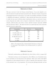
Qin and BhadeshiaPhase field methodtend to have narrow composition ranges (free energyincreases with deviation from stoichiometry). An exampleis that in a simulation of Al–2 wt-%Si solidification,the thickness of interface between primary aluminiumrich dendrites and liquid had a maximum of about2l56?5 nm but had to be restricted to ,0?2 nm for thatbetween silicon particles and the liquid. 20 This is toensure that a realistic interfacial energy is obtained, butthe small width dramatically increases the computationaleffort.Others 20–22 have assumed that the phase compositionsinside the interface are governed by the equationLg aLc a ~ LgbLc b (7)and have mistakenly identified these derivatives withchemical potential LG/Ln, where G is the total chemicalfree energy of the phase concerned and n the number ofmoles of the solute concerned. It is of course gradients inthe chemical potential which govern diffusion so it may bemisleading to call the derivatives in equation (7) the phasediffusion potential. 23 Note also that equation (7) does notreduce to an equilibrium condition when the chemicalpotential is uniform in the parent and product phases.When equation (7) is applied in phase field modelling, ithas been suggested 23 that because the gradients in Lg/Lc donot reduce to zero even at equilibrium, it is necessary tocompensate for this by some additional component to thefree energy density g, which might be interpreted in termsof the structure of the interface. However, this is arbitraryand as has been pointed out previously, 23 difficulties arisewhen the interface width in the simulation is greater thanthe physical width.Thermodynamics of irreversibleprocessesThe determination of the rate of change requiresultimately a relationship between time, the free energydensity and the order parameter. The approach in sharpinterface models is usually atomistic, with activationenergies for the rate controlling process and someconsideration of the structure of the interface inpartitioning the driving force between the variety ofpossible dissipative processes. The phase field methodhas no such detail, but rather relies on a fundamentalapproximation of the thermodynamics of irreversibleprocesses, 24–27 that the flux describing the rate isproportional to the force responsible for the change.For irreversible processes the equations of classicalthermodynamics become inequalities. For example, atthe equilibrium melting temperature, the free energies ofthe pure liquid and solid are identical (G liquid 5G solid ) butnot so below that temperature (G liquid .G solid ).The thermodynamics of irreversible processes dealswith systems which are not at equilibrium but arenevertheless stationary. It deals, therefore, with steadystate processes where free energy is being dissipatedmaking the process irreversible in the language ofthermodynamics since after the application of aninfinitesimal force, the system then does not revert toits original state on removal of that force.The rate at which energy is dissipated in anirreversible process is the product of the temperatureand the rate of entropy production (T : S) withT : S~JX or for multiple processes, T : S~ X iJ i X i (8)where J is a generalised flux of some kind, and X ageneralised force (Table 1).Given equation (8), it is often found experimentallythat the flux is proportional to the force (J!X); familiarexamples include Ohm’s law for electrical current flowand Fourier’s law for heat diffusion. When there aremultiple forces and fluxes, each flow J i is related linearlynot only to its conjugate force X i , but also is relatedlinearly to all other forces present (J i 5M ij X j )i,j51,2,3…; thus, the gradient in the chemical potentialof one solute will affect the flux of another. It isemphasised here that the linear dependence described isnot fundamentally justified other than by the fact that itworks. The dependence can be recovered by a Taylorexpansion of J{X} about equilibrium where X50JfXg~Jf0gzJ’ f0g X 21! zJ’’ f0gX2! ...J{0}50 since there is no flux at equilibrium. Theproportionality of J to X is obtained when all termsbeyond the second are neglected. The important point isthat the approximation is only valid when the forces aresmall. There is no phase field model that the authors areaware of which considers higher order terms in therelation between J and X.Implementation in rate equationsNon-conserved order parameterThe dissipation of free energy as a function of time in anirreversible process must satisfy the inequalitydG¡0 (9)dtas the system approaches equilibrium. When there aremultiple processes occurring simultaneously, it is onlythe overall condition which needs to be satisfied ratherthan for each individual process; an expansion ofequation (9) gives dG Lwdwc,TLtz dG LTdT Ltw,cz dGc,Tdcw,T LcLtw,T¡0 (10)w,cbut to ensure that the free energy of the system decreasesmonotonically with time, it is sufficient thatTable 1Forcee.m.f. : LyLz{ 1 LTT Lz{ Lm iLzStressExamples of forces and their conjugate fluxes*FluxElectrical CurrentHeat fluxDiffusion fluxStrain rate*z is distance, y is the electrical potential in volts, and m is achemical potential. ‘e.m.f.’ stands for electromotive force.806 Materials Science and Technology 2010 VOL 26 NO 7