Phase Field Modelling - Department of Materials Science and ...

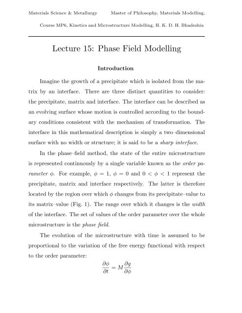
Materials Science & MetallurgyMaster of Philosophy, Materials Modelling,Course MP6, Kinetics and Microstructure Modelling, H. K. D. H. BhadeshiaLecture 15: Phase Field ModellingIntroductionImagine the growth of a precipitate which is isolated from the matrixby an interface.There are three distinct quantities to consider:the precipitate, matrix and interface. The interface can be described asan evolving surface whose motion is controlled according to the boundaryconditions consistent with the mechanism of transformation. Theinterface in this mathematical description is simply a two–dimensionalsurface with no width or structure; it is said to be a sharp interface.In the phase–field method, the state of the entire microstructureis represented continuously by a single variable known as the order parameterφ. For example, φ = 1, φ = 0 and 0

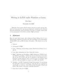
Fig. 1: (a) Sharp interface. (b) Diffuse interface.where M is a mobility. The term g describes how the free energy variesas a function of the order parameter; at constant T and P , this takesthe typical form (Appendix 1)†:∫g =V[g 0 {φ, T } + ɛ(∇φ) 2 ]dV (1)where V and T represent the volume and temperature respectively. Thesecond term in this equation depends only on the gradient of φ and henceis non–zero only in the interfacial region; it is a description therefore ofthe interfacial energy. The first term is the sum of the free energies ofthe precipitate and matrix, and may also contain a term describing theactivation barrier across the interface. For the case of solidification,g 0 = hg S + (1 − h)g L + Qfwhere g S and g L refer to the free energies of the solid and liquid phases† If the temperature varies then the functional is expressed in termsof entropy rather than free energy.

espectively, Q is the height of the activation barrier at the interface,h = φ 2 (3 − 2φ) and f = φ 2 (1 − φ) 2Notice that the term hg S + Qf vanishes when φ =0(i.e. only liquid ispresent), and similarly, (1 − h)g L + Qf vanishes when φ =1(i.e. onlysolid present). As expected, it is only when both solid and liquid arepresent that Qf becomes non–zero. The time–dependence of the phasefield then becomes:∂φ∂t = M[ɛ∇2 φ + h ′ {g L − g S }−Qf ′ ]The parameters Q, ɛ and M have to be derived assuming some mechanismof transformation.Two examples of phase–field modelling are as follows: the first iswhere the order parameter is conserved. With the evolution of compositionfluctuations into precipitates, it is the average chemical compositionwhich is conserved. On the other hand, the order parameter is not conservedduring grain growth since the amount of grain surface per unitvolume decreases with grain coarsening.Cahn–Hilliard Treatment of Spinodal DecompositionIn this example, the order parameter is the chemical composition.In solutions that tend to exhibit clustering (positive ∆H M ), it is possiblefor a homogeneous phase to become unstable to infinitesimal perturbationsof chemical composition. The free energy of a solid solution whichis chemically heterogeneous can be factorised into three components.

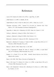
First, there is the free energy of a small region of the solution in isolation,given by the usual plot of the free energy of a homogeneous solutionas a function of chemical composition.The second term comes about because the small region is surroundedby others which have different chemical compositions. Fig. 2shows that the average environment that a region a feels is different (i.e.point b) from its own chemical composition because of the curvature inthe concentration gradient. This gradient term is an additional free energyin a heterogeneous system, and is regarded as an interfacial energydescribing a “soft interface” of the type illustrated in Fig. 1b. In thisexample, the soft–interface is due to chemical composition variations,but it could equally well represent a structural change.Fig. 2: Gradient of chemical composition. Point arepresents a small region of the solution, point b theaverage composition of the environment around pointa, i.e. the average of points c and d.The third term arises because a variation in chemical compositionalso causes lattice strains in the solid–state. We shall assume here thatthe material considered is a fluid so that we can neglect these coherency

strains.The free energy per atom of an inhomogeneous solution is given by(Appendix 1):∫g ih =V[g{c 0 } + v 3 κ(∇c) 2 ]dV (2)where g{c 0 } is the free energy per atom in a homogeneous solution ofconcentration c 0 , v is the volume per atom and κ is called the gradientenergy coefficient. g ih is often referred to as a free energy functional sinceit is a function of a function. See Appendix 1 for a detailed derivation.Equilibrium in a heterogeneous system is then obtained by minimisingthe functional subject to the requirement that the average concentrationis maintained constant:∫(c − c 0 )dV =0where c 0 is the average concentration. Spinodal decomposition cantherefore be simulated on a computer using the functional defined inequation 2. The system would initially be set to be homogeneous butwith some compositional noise. It would then be perturbed, allowingthose perturbations which reduce free energy to survive. In this way, thewhole decomposition process can be modelled without explicitly introducingan interface. The interface is instead represented by the gradientenergy coefficient. For a simulation, seewww.msm.cam.ac.uk/phase − trans/mphil/spinodal.movie.htmlA theory such as this is not restricted to the development of compositionwaves, ultimately into precipitates. The order parameter can

e chosen to represent strain and hence can be used to model phasechanges and the associated microstructure evolution.In the phase field modelling of solidification, there is no distinctionmade between the solid, liquid and the interface. All regions are describedin terms of the order parameter. This allows the whole domainto be treated simultaneously. In particular, the interface is not trackedbut is given implicitly by the chosen value of the order parameter as afunction of time and space. The classical formulation of the free boundaryproblem is replaced by equations for the temperature and phasefield.Appendix 1Recall (MP4–6) that a Taylor expansion for a single variable aboutX = 0 is given byJ{X} = J{0} + J ′ {0} X 1! + J ′′ {0} X22!...A Taylor expansion like this can be generalised to more than one variable.Cahn assumed that the free energy due to heterogeneities in asolution can be expressed by a multivariable Taylor expansion:g{y, z, . . .} =g{c 0 } + y ∂g∂y + z ∂g∂z + ...+ 1 []y 2 ∂2 g2 ∂y 2 + z2 ∂2 g∂z 2 +2yz ∂2 g∂y∂z + ... + ...in which the variables, y, z, . . . in our context are the spatial compositionderivatives (dc/dx, d 2 c/dx 2 , etc). For the free energy of a small volumeelement containing a one–dimensional composition variation (and

neglecting third and high–order terms), this givesdcg = g{c 0 } + κ 1dx + κ d 2 ( ) 2c dc2dx 2 + κ 3(3)dxwhere c 0 is the average composition.∂gwhere κ 1 =∂(dc/dx)∂gκ 2 =∂(d 2 c/dx 2 )κ 3 = 1 2∂ 2 g∂(dc/dx) 2In this, κ 1 is zero for a centrosymmetric crystal since the free energymust be invariant to a change in the sign of the coordinate x.The total free energy is obtained by integrating over the volume:∫g T =V[d 2 ( ) 2 ]c dcg{c 0 } + κ 2dx 2 + κ 3dxOn integrating the third term in this equation by parts†:∫d 2 ∫cκ 2dx 2 = κ dc2dx − dκ2dc(4)( ) 2 dcdx (5)dxAs before, the first term on the right is zero, so that an equation of theform below is obtained for the free energy of a heterogeneous system:∫g =V[g 0 {φ, T } + ɛ(∇φ) 2 ]dV (6)†∫∫uv ′ dx = uv −u ′ v dx

References1. J. W. Cahn: Trans. Metall. Soc. AIME 242 (1968) 166–179.2. J. E. Hilliard: Phase Transformations, ASM International, MaterialsPark, Ohio, USA (1970) 497–560.3. J. A. Warren: IEEE Computational Science and Engineering (Summer1995) 38–49.4. A. A. Wheeler, G. B McFadden and W. J. Boettinger: Proc. R. Soc.London A 452 (1996) 495–525.5. J. W. Cahn and J. E. Hilliard: Journal of Chemical Physics 31 (1959)688–699.6. J. W. Cahn: Acta Metallurgica 9 (1961) 795–801.7. A. A. Wheeler, B. T. Murray and R. J. Schaefer: Physica D 66 (1993)243–262.8. M. Honjo and Y. Saito: ISIJ International 40 (2000) 916–921.9. M. Ode, S. G. Kim and T. Suzuki: ISIJ International 41 (2001) 1076–1082.

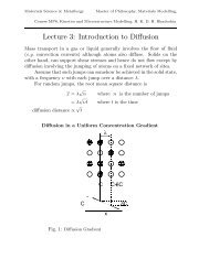
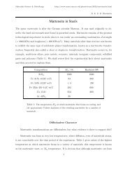
REVIEWPhase field methodR. S. Qin 1 and H. K. Bhadeshia* 2In an ideal scenario, a phase field model is able to compute quantitative aspects of the evolutionof microstructure without explicit intervention. The method is particularly appealing because itprovides a visual impression of the development of structure, one which often matchesobservations. The essence of the technique is that phases and the interfaces between the phasesare all incorporated into a grand functional for the free energy of a heterogeneous system, usingan order parameter which can be translated into what is perceived as a phase or an interface inordinary jargon. There are, however, assumptions which are inconsistent with practicalexperience and it is important to realise the limitations of the method. The purpose of this reviewis to introduce the essence of the method, and to describe, in the context of materials science, theadvantages and pitfalls associated with the technique.Keywords: Phase field models, Structural evolution, Multiphase, Multicomponent, Gradient energyIntroductionThe phase field method has proved to be extremelypowerful in the visualisation of the development ofmicrostructure without having to track the evolution ofindividual interfaces, as is the case with sharp interfacemodels. The method, within the framework of irreversiblethermodynamics, also allows many physicalphenomena to be treated simultaneously. Phase fieldequations are quite elegant in their form and clear for allto appreciate, but the details, approximations andlimitations which lead to the mathematical form areperhaps not as transparent to those whose primaryinterest is in the application of the method. Thematerials literature in particular thrives in comparisonsbetween the phase field and classical sharp interfacemodels which are not always justified. The primarypurpose of this review is to present the method in a formas simple as possible, but without avoiding a few of thederivations which are fundamental to the appreciationof the method. Example applications are not particularlycited because there are other excellent reviews andarticles which contain this information together withdetailed theory, for example, Refs. 1–7.Imagine the growth of a precipitate which is isolatedfrom the matrix by an interface. There are three distinctentities to consider: the precipitate, matrix and interface.The interface can be described as an evolving surface whosemotion is controlled according to the boundary conditionsconsistent with the mechanism of transformation. Theinterface in this mathematical description is simply a twodimensionalsurface; it is said to be a sharp interface whichis associated with an interfacial energy s per unit area.1 Graduate Institute of Ferrous Technology Pohang University of Scienceand Technology Pohang 790 784, Korea2 University of Cambridge Materials Science and Metallurgy PembrokeStreet, Cambridge CB2 3QZ, UK*Corresponding author, email hkdb@cam.ac.ukIn the phase field method, the state of the entiremicrostructure is represented continuously by a singlevariable known as the order parameter w. Forexample,w51, w50and0,w,1representtheprecipitate,matrixandinterface respectively. The latter is therefore located by theregion over which w changes from its precipitate value to itsmatrix value (Fig. 1). The range over which it changes is thewidth of the interface. The set of values of the orderparameter over the whole volume is the phase field. Thetotal free energy G of the volume is then described in termsof the order parameter and its gradients, and the rate atwhich the structure evolves with time is set in the context ofirreversible thermodynamics, and depends on how G varieswith w. Itisthegradientsinthermodynamicvariablesthatdrive the evolution of structure.Consider a more complex example, the growth of agrain within a binary liquid (Fig. 2). In the absence of fluidflow, in the sharp interface method, this requires thesolution of seven equations involving heat and solutediffusion in the solid, the corresponding processes inthe liquid, energy conservation at the interface and theGibbs–Thomson capillarity equation to allow for the effectof interface curvature on local equilibrium. The number ofequations to be solved increases with the number ofdomains separated by interfaces and the location of eachinterface must be tracked during transformation. This maymake the computational task prohibitive. The phase fieldmethod clearly has an advantage in this respect, with asingle functional to describe the evolution of the phasefield, coupled with equations for mass and heat conduction,i.e. three equations in total, irrespective of the numberof particles in the system. The interface illustrated inFig. 2b simply becomes a region over which the orderparameter varies between the values specified for thephases on either side. The locations of the interfaces nolonger need to be tracked but can be inferred from the fieldparameters during the calculation.Notice that the interface in Fig. 2b is drawn as a regionwith finite width, because it is defined by a smooth variationß 2010 Institute of Materials, Minerals and MiningPublished by Maney on behalf of the InstituteReceived 6 April 2009; accepted 20 April 2009DOI 10.1179/174328409X453190 Materials Science and Technology 2010 VOL 26 NO 7 803

Qin and BhadeshiaPhase field method1 a sharp interface and b diffuse interfacein w between w50 (solid)andw51 (liquid).Theorderparameter does not change discontinuously during thetraverse from the solid to the liquid. The position of theinterface is fixed by the surface where w50?5. The mathematicalneed for this continuous change in w to define theinterface requires that it has a width (2l), and therein liesone of the problems of phase field models. Boundariesbetween phases in real materials tend, with few exceptions,to be at most a few atoms in width, as defined for exampleby the extent of the strain field of interfacial dislocations.Phase–field models can cope with narrow boundaries, butthe computational time t scales with interface thickness ast/t 0 !(l/l 0 ) 2D where D represents the dimension of thesimulation. Defining a broader interface reduces the computationalresources required, but there is a chance thatdetail is lost, for example at the point marked ‘P’ in Fig. 2.There are ways of using adaptive grids in which thegrid spacing is finer in the vicinity of the interface,assuming that w varies significantly only in the regionnear the interface. 8 This approach is useful if most of thefield is uniform, or when interfaces occupy only a smallportion of the volume, for example when considering asingle thermal dendrite growing in a matrix. It is lessuseful when there are many particles involved since theextent of uniformity then decreases.Order parameterThe order parameters in phase field models may ormay not have macroscopic physical interpretations. Fortwo-phase materials, w is typically set to 0 and 1 for theindividual phases, and the interface is the domain where0,w,1. For the general case of N phases present in amatrix, there will be a corresponding number of phasefield order parameters w i with i51 to N. w i 51 thenrepresents the domain where phase i exists, w i 50 where itis absent and 0,w i ,1 its bounding interfaces. Supposethat the matrix is represented by w 0 then it is necessarythat at any locationX Ni~0w i ~1 (1)It follows that the interface between phases 1 and 2,where 0,w 1 ,1 and 0,w 2 ,1 is given by w 1 zw 2 51;similarly, for a triple junction between three phaseswhere 0,w i ,1 for i51,2,3, the junction is the domainwhere w 1 zw 2 zw 3 51.The order parameter can also be expressed as avector function, for example in representing the variationof interfacial energy as a function of interfaceorientation 9–11 and this kind of theory has been used inthe phase field modelling of crystal shapes, for example,Refs. 12 and 13.ThermodynamicsThe thermodynamic function of state selected for thephase field simulation depends on the definition of theproblem. Entropy is appropriate for an isolated system(a)a sharp interface model; b phase field model2 Solidification(b)804 Materials Science and Technology 2010 VOL 26 NO 7

Qin and BhadeshiaPhase field methodwhich is not isothermal, the Gibbs free energy isappropriate for an isothermal system at constantpressure, and the Helmholtz free energy when temperatureand volume are kept constant. The remainder of thediscussion is in terms of the Gibbs free energy, which isknowable for a homogeneous phase, but is required fora heterogeneous system in which the order parameter isnot uniform. Cahn and Hilliard developed the necessarytheory by considering a multivariate Taylor expansion.14–17 Writing g 0 {w, c, T} as the free energy per unitvolume of a homogeneous phase of composition c attemperature T, and the corresponding term for aheterogeneous system as g, the Taylor expansion givesg~g 0 z Lg 0L+w +wz1 L 2 g 02L(+w) 2L(+w)2 z ...z Lg 0L+ 2 w L+2 wz 1 L 2 g 02L(+ 2 w) 2(+2 w) 2 z ...z Lg 0L+c +cz1 L 2 g 02L(+c) 2L(+c)2 z ...z Lg 0L+ 2 c L+2 cz 1 L 2 g 02L(+ 2 c) 2(+2 c) 2 z ...z Lg 0L+T +Tz 1 L 2 g 02L(+T) 2L(+T)2 z ...z Lg 0L+ 2 T L+2 Tz 1 L 2 g 02L(+ 2 T) 2(+2 T) 2z ...z 1 2L 2 g 0L+wL+c +w+cz L2 g 0L+wL+T +w+Tz L2 g 0L+cL+T +c+Tz ... !z ... (2)The coefficients of odd orders of differentiation must beset to zero since the free energy must be invariant to achange in the sign of the coordinate. Integration by partscan be used to achieve further simplification sinceðVLg 0L+ 2 w dr~ Lg ð0L+ 2 w ^n : +w{VLLwLg 0L+ 2 w(+w) 2 dr (3)where ^n is a unit vector along the coordinate. The first (odd)term on the right again reduces to zero, whereas the secondterm is combined with an existing (+w) 2 term in equation(2). Similar procedures apply to the terms containing+ 2 c and + 2 T. Since the diffusion length of solute andparticularly of heat are generally large, their spatialgradients are likely to be small so that +T(+c(+w(There are of course circumstances where concentrationgradients are the key phenomena studied, such as inspinodal decomposition, in which case the solute gradientterm clearly must be retained). Taking this into account andlimiting the Taylor expansion to first and second orderterms, it follows that the free energy for a heterogeneoussystem is given by integrating over the volume Vð G~ fw,c,Tgz e2 2 (+w)2 dV (4)Vg 0where g 0 is the free energy per unit volume,e 2 ~L 2 g 0 =L(+w) 2 {2L(Lg 0 =L+ 2 w)=Lw is the gradient energycoefficient. In actual computations e is determined in such away as to give an accurate description of interfaceproperties such as the energy per unit area and anisotropyof interfacial energy, as described later.It is useful to comment further on g 0 {w, c, T} inheterogeneous materials. Consider a phase b (w51)growing in a (w50) and with 0,w,1 defining the a–binterface. g 0 is likely to be known for the homogeneousphases a and b but not for the interface region given acontinuous variation in concentration over this region,into which the free energy density must somehow beextrapolated. Any general expression for g 0 covering theentire domain of order parameter (0(w(1) must at thesame time reduce to the appropriate term when only onephase is present. There are versatile expressions suggestedin the literature for g 0 , usually assuming a doublewell potential shape 18 with the two minima correspondingto the a and b phasesfw,c,Tg~hfwgg0 a f ca ,Tgz(1{hfwg)g b 0 cb ,Tg 0z 14v w2 (1{w) 2 (5)where h5w 3 (6w 2 215wz10), 19 and g0 a and gb 0are the freeenergy densities of the respective phases; c a and c b aresimilarly the solute contents of these phases. v is acoefficient which can be adjusted to fit the desiredinterfacial energy but has to be positive to be consistentwith a double well potential as opposed to one with twopeaks. The third term on the right in equation (5) is asymmetrical double well. h{w} is a monotonic functionsuch that h{0}50 and h{1}51 so that the free energies ofbulk a and b phases are reproduced. The first two terms onthe right hand side of equation (5) generate the possibleasymmetry. Because g 0 may contain assumptions inconsistentwith real data, e has to be modified accordingly toreproduce the correct interface properties.Equation (5) is sufficient for computing transitionswhich do not involve a change in composition. For thecase where solute is partitioned during transformation, itbecomes difficult to specify the nature of the interfacialregion where the order parameter is neither 1 nor 0. Thesolute content c I within the interface will vary monotonicallybetween the limits of the concentrations in thephases (w50,1, c a and c b respectively) in contact with theinterfacial region. Suppose that the interface is consideredto be a (heterogeneous) phase in its own right,and assumed to be composed of a mixture of a and b, ofsolute concentrations c a I and cb I, then the compositionsof these phases within the interface will vary withposition ifc I ~hfwgc a I fwgz(1{hfwg)c b Ifwg (6)The question then arises as to what determines c a I and cb Ibecause these quantities are necessary not simply to setthe variation in c I with position within the interface, butalso to calculate the corresponding variation in freeenergy. For a given interface thickness, this leads to thedefinition of the excess energy of the interfacial region,which can then be compared directly with independentmeasurements of interfacial energy per unit area. Theexperimental data set the upper limit to the interfacethickness in a phase field simulation.A simple assumption in the past has been to takec a I ~cb I ~c I particularly where the phases concerned aresolutions, i.e. their free energy does not vary sharplywith solute content, even though this would lead tounequal chemical potentials. Phase field simulations ofsolidification involving such phases in the Cu–Ni systemhave used large interface thicknesses of about 2l518 nmwithout compromising details of the dendrite patterns. 19Difficulties arise when dealing with compounds whichMaterials Science and Technology 2010 VOL 26 NO 7 805

Qin and BhadeshiaPhase field methodtend to have narrow composition ranges (free energyincreases with deviation from stoichiometry). An exampleis that in a simulation of Al–2 wt-%Si solidification,the thickness of interface between primary aluminiumrich dendrites and liquid had a maximum of about2l56?5 nm but had to be restricted to ,0?2 nm for thatbetween silicon particles and the liquid. 20 This is toensure that a realistic interfacial energy is obtained, butthe small width dramatically increases the computationaleffort.Others 20–22 have assumed that the phase compositionsinside the interface are governed by the equationLg aLc a ~ LgbLc b (7)and have mistakenly identified these derivatives withchemical potential LG/Ln, where G is the total chemicalfree energy of the phase concerned and n the number ofmoles of the solute concerned. It is of course gradients inthe chemical potential which govern diffusion so it may bemisleading to call the derivatives in equation (7) the phasediffusion potential. 23 Note also that equation (7) does notreduce to an equilibrium condition when the chemicalpotential is uniform in the parent and product phases.When equation (7) is applied in phase field modelling, ithas been suggested 23 that because the gradients in Lg/Lc donot reduce to zero even at equilibrium, it is necessary tocompensate for this by some additional component to thefree energy density g, which might be interpreted in termsof the structure of the interface. However, this is arbitraryand as has been pointed out previously, 23 difficulties arisewhen the interface width in the simulation is greater thanthe physical width.Thermodynamics of irreversibleprocessesThe determination of the rate of change requiresultimately a relationship between time, the free energydensity and the order parameter. The approach in sharpinterface models is usually atomistic, with activationenergies for the rate controlling process and someconsideration of the structure of the interface inpartitioning the driving force between the variety ofpossible dissipative processes. The phase field methodhas no such detail, but rather relies on a fundamentalapproximation of the thermodynamics of irreversibleprocesses, 24–27 that the flux describing the rate isproportional to the force responsible for the change.For irreversible processes the equations of classicalthermodynamics become inequalities. For example, atthe equilibrium melting temperature, the free energies ofthe pure liquid and solid are identical (G liquid 5G solid ) butnot so below that temperature (G liquid .G solid ).The thermodynamics of irreversible processes dealswith systems which are not at equilibrium but arenevertheless stationary. It deals, therefore, with steadystate processes where free energy is being dissipatedmaking the process irreversible in the language ofthermodynamics since after the application of aninfinitesimal force, the system then does not revert toits original state on removal of that force.The rate at which energy is dissipated in anirreversible process is the product of the temperatureand the rate of entropy production (T : S) withT : S~JX or for multiple processes, T : S~ X iJ i X i (8)where J is a generalised flux of some kind, and X ageneralised force (Table 1).Given equation (8), it is often found experimentallythat the flux is proportional to the force (J!X); familiarexamples include Ohm’s law for electrical current flowand Fourier’s law for heat diffusion. When there aremultiple forces and fluxes, each flow J i is related linearlynot only to its conjugate force X i , but also is relatedlinearly to all other forces present (J i 5M ij X j )i,j51,2,3…; thus, the gradient in the chemical potentialof one solute will affect the flux of another. It isemphasised here that the linear dependence described isnot fundamentally justified other than by the fact that itworks. The dependence can be recovered by a Taylorexpansion of J{X} about equilibrium where X50JfXg~Jf0gzJ’ f0g X 21! zJ’’ f0gX2! ...J{0}50 since there is no flux at equilibrium. Theproportionality of J to X is obtained when all termsbeyond the second are neglected. The important point isthat the approximation is only valid when the forces aresmall. There is no phase field model that the authors areaware of which considers higher order terms in therelation between J and X.Implementation in rate equationsNon-conserved order parameterThe dissipation of free energy as a function of time in anirreversible process must satisfy the inequalitydG¡0 (9)dtas the system approaches equilibrium. When there aremultiple processes occurring simultaneously, it is onlythe overall condition which needs to be satisfied ratherthan for each individual process; an expansion ofequation (9) gives dG Lwdwc,TLtz dG LTdT Ltw,cz dGc,Tdcw,T LcLtw,T¡0 (10)w,cbut to ensure that the free energy of the system decreasesmonotonically with time, it is sufficient thatTable 1Forcee.m.f. : LyLz{ 1 LTT Lz{ Lm iLzStressExamples of forces and their conjugate fluxes*FluxElectrical CurrentHeat fluxDiffusion fluxStrain rate*z is distance, y is the electrical potential in volts, and m is achemical potential. ‘e.m.f.’ stands for electromotive force.806 Materials Science and Technology 2010 VOL 26 NO 7

Qin and BhadeshiaPhase field method dGdwc,T LwLt¡0 (11)c,TIf it is now assumed from the approximations in thetheory of irreversible thermodynamics that the ‘flux’ isproportional to the ‘force’ then LwdG~{M w(12)Ltc,T|fflfflfflffl{zfflfflfflffl}fluxdwc,T|fflfflfflfflffl{zfflfflfflfflffl}forceThis gives" # 2dG{M w ¡0, i:e:, M w ¢0 (13)dwc,Tso that the mobility M must be positive or zero. It can beshown that 28dGdw ~ LgLw {e2 w +2 wso that LwLt ~M we 2 w +2 w{ LgfwgLw(14)The equation on the right is a generic form for theevolution of a non-conserved order parameter in amanner which leads to the reduction of free energy.Conserved order parameterSome order parameters are conserved during evolutionwhereas others need not be. For example, when wdescribes solidification the integrated value of w over thewhole phase field will not be the same once solidificationis completed. In such a case, equation (12) is sufficient toinitiate a phase field calculation. On the other hand,solute must be conserved during a diffusion process. Theauthors illustrate this with the classical example of solutediffusion, where the equivalent of equation (4) is 29ð G~ gfgz c1 2 e2 c (+c)2 dV (15)Vbut because concentration is a conserved quantity, it isnecessary to also satisfyLcLt ~+: J c (16)where J c is the solute flux. From the appropriate termfor solute in equation (10), substituting for Lc/Lt, theauthors see thatdGdcw,T|(+ : J c )¡0LcLt¡0 is equivalent to dGw,Tdcand given the identity B+ : A:+ : (AB){A : +Bit follows that" # {+ : dGJ c zJ c:dG + ¡0 (17)dcw,Tdcw,T|fflfflfflfflfflfflfflfflfflfflfflfflfflffl{zfflfflfflfflfflfflfflfflfflfflfflfflfflffl}~0The term on the left is identified to be zero because therecan be no flux through the bounding surface of a closedsystem (G is an integral over volume, which by theGauss theorem, can be expressed as an integral over itsw,Tbounding surface). A combination of equations (17) and(16) givesLcLt ~+: M c + dG (18)dcw,Twhere M c is the diffusional mobility and dG/dc is thevariational derivative of G with respect to c. The sameassumption applies here as emphasised in the derivationof equation (12) that the force and flux are assumed tobe linearly dependent.If the gradient energy can be neglected then in abinary alloy the term dG/dc corresponds to thedifference in the chemical potentials of the twocomponents. 30The general theory that describes governing equationsfor various types of order parameters has been reviewedin detail by Hohenberg and Halperin. 31Parameter specificationIn order to apply the phase field equations, it isnecessary to know the mobility M, gradient energycoefficient e and the interfacial fitting parameter v inorder to utilise the phase field method.The interfacial energy per unit area s is derived fromthe excess free energy density associated with theinterfacial region. 32 The following derivation due toWheeler 11 is for the case where w is not conserved. Sincethe authors focus on the interfacial region only,equation (5) reduces to g 0 fwg~ 14v w2 (1{w) 2 . At equilibriumsince Lw/Lt50, the one-dimensional form ofequation (14) becomese 2d2 w fwgdx 2{Lg Lw ~0which on integration gives e2 2 dw 2{gfwg~0 (19)dxw with its origin redefined at the centre of the interface isdesignated w 0 ; an exact solution to equation (19) 11showing the smooth variation in the order parameterbetween its bulk values is( " #)w 0 ~ 1 2 1ztanh x2(2v) 1=2 eso that the interface thickness 2l~4(2v) 1=2 e (20)The authors note that with the assumptions outlined, thethickness of the interface is proportional to the gradientenergy coefficient. The energy of the interface per unitarea is then given by integrating equation (19)ð z? s~ e 2 dw 20dx~ (2)1=2 e(21){? dx 12(v) 1=2The width of the interface 2l is treated as a parameterwhich is adjusted to minimise computational expense orusing some other criterion such as the resolution ofdetail in the interface. Values of the interfacial energyper unit area s may be available from experimentalmeasurements. Given these two quantities, the expressionsfor interfacial energy and interfacial width canbe solved simultaneously to yield e and v. Both of theterms in equation (19) contribute to the interface energy,Materials Science and Technology 2010 VOL 26 NO 7 807

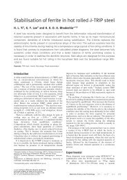
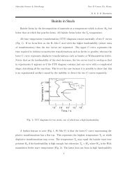
Qin and BhadeshiaPhase field methodi.e. through the existence of gradients in the orderparameter and because the free energy density there isdefined to be different from that of the bulk phases.The mobility M is determined experimentally, forexample in a single component system, by relating theinterface velocity v to driving force DG using chemicalrate theory in which v5M6DG. 27 In simulatingspinodal decomposition, diffusion data and thermodynamicscan be used to obtain mobilities. When themodels are used simply for illustrating the generalprinciples of morphological evolution, the mobility isoften fixed by trial and error. Too large a mobility leadsto numerical instabilities and the computing timebecomes intolerable if the mobility is set to be too small.Numerical procedures andinterpretationsThe governing equations of phase fields are usuallysolved using the finite difference or finite elementtechniques. The following discussion will for simplicityfocus on the explicit finite difference method at twodimensionalsquare regular lattices. The lattice spacingDx is then uniform and set so that the interface isdescribed by at least four cells in order to capturemoderate detail in the interface. As in all numericalmethods, coarse spacings may not have sufficientresolution to deal with the problem posed, and maylead to numerical instabilities. The discrete time step isaccordingly set such that Dtv 1 2 (Dx)2 =D where D is thelargest of all included solute and heat diffusivities.An interesting aspect of using a value of Dx which islarge relative to the detail in the microstructure is thatnoise, to a level of ,1%, is introduced into the system. Itis found, in the absence of such noise, that dendrites inpure systems tend to grow without side-branching; 1,33expressed differently, a fine Dx leads to needle-likedendrites without side branches. This confirms othertheory which suggests that small perturbations correspondingto thermal noise are responsible for the sidebranchingdendrites. 8,34,35The finite element lattice has to be initialised withvalues of w, c and T but sharp changes in w should beavoided to prevent calculation instabilities. The initialconfiguration should also account for boundary conditionsand this may necessitate the introduction of aghost layer of lattices compatible with the boundaryconditions. There is no simple method of introducingheterophase fluctuations of the kind associated withclassical nucleation theory. But the latter can be used tocalculate the appropriate number of nuclei and implementthem on to the lattice.It is normal, for the sake of computational stability, touse dimensionless variables in the governing equationsso that the occurrence of very small or very largenumbers is avoided D x~Dx=L ~ c , D t!D ~ x ~ 2 ~=D c , M w ~L 2 c RT c=D c V m , e~e(V ~ m =RT c ) 1=2 =L c , v~vRT ~ c =V m and~g a { g ~ b ~(g a {g b )V m =RT c , where L c is a characteristiclength, T c a characteristic temperature (for example atransition temperature) and V m is the molar volume.After expressing the variables in this way, they rangeroughly between 0 and 1. The variables are unnormalisedwhen interpreting the outputs of the model. It maybe necessary in some cases to introduce fluctuations,which can be conducted by disturbing the driving forcerather than the variables such as solute concentration ortemperature in order to avoid the violation of conservationconditions by the fluctuations.Comparison with overall transformationkinetics modelsAttempts have been made to compare and contrast theoverall transformation kinetics theory invented byKolmogorov in its most general form 36 and alsodeveloped by Avrami, 37–39 Johnson and Mehl 40 (thistheory is henceforth referred to using the acronymKJMA). The essence of the method is that given thenucleation and growth rates of particles forming from aparent phase in a volume, the total extended volume Veaof a particles can be calculated first without accountingfor impingement, and then a correct volume V a isobtained by multiplying the extended fraction by theprobability of finding untransformed material (i.e. thefraction (12V a /V) of the parent phase that remains)where V is the total volume, so thatdV a ~ 1{ V a dVea Vwhich on integration gives V a V ~1{exp { V ea (22)VThis conversion between extended and real spacepermits hard impingement to be taken into account,and requires an assumption that the volume of anarbitrary transformed crystal is much smaller than thatof the total volume. In addition, it is assumed that nucleiwill develop at random sites because the conversionrelies on probabilities. Nevertheless, grain boundarynucleation can be treated as in Ref. 41 and this methodhas in practice been applied with useful results. 42 Thereis a huge variety of equations that result depending onthe specific mechanisms of transformation; these havebeen reviewed by Christian. 43For two-dimensional growth at a rate G of initiallyspherical particles beginning with a constant number ofsites N 0 which can develop from time t50 into particles,equation (22) becomesV a V ~1{exp { N 0G 2 4pt2(23)Jou and Lusk 44 attempted to compare this equation witha phase field which was designed to emulate sphericalparticles growing in the manner described by equation(23). The comparison is approximate because theywere not able to suppress capillarity effects in the phasefield model, which resulted in slower growth at smallparticle size, so that the phase field model underestimatedrelative to equation (23). Capillarity can ofcourse be included in equations based on overalltransformation kinetics, 45–49 but this was not taken intoaccount in making the comparison.Jun and Lusk also examined an extreme scenario inwhich a single particle is placed at the centre of a squareparent phase, and modelled transformation using thephase field method and a geometrical exact-solution.The results, shown in Fig. 3, seem to suggest that theKJMA method fails since it predicts a slower evolutionof phase fraction when compared with the exactanalytical solution and the phase field technique. The808 Materials Science and Technology 2010 VOL 26 NO 7

Qin and BhadeshiaPhase field methoda particle located at centre of square, growing radially and impinging with boundary of square; b comparison of overallkinetics calculated using equation (23), phase field model and exact analytical solution (latter two are plotted as singlecurve since they gave similar results)3 Single particle growth: data from Ref. 44KJMA method relies on randomness – had the particlebeen placed anywhere other than the centre, impingementwould have occurred earlier. Furthermore, asstated earlier, the theory requires the growing particle tobe much smaller than the volume of the material as awhole. 36,50 While it is true that impingement effects arelikely to underestimate the fraction of transformationwhen there are very few particles present and whichgrow to consume large fractions of the matrix, this is nota realistic scenario for applications where real microstructuralevolution is calculated.The most obvious difference between the mechanisticKJMA method and the phase field method, in which it isdifficult to incorporate atomistic information, is that thelatter allows the structure to be pictured as it evolves.This is not possible for the KJMA method given itsreliance on probabilities and the conversion betweenextended and real space. In suitably chosen problems,the phase field method can better account for phenomenain which there is an overlap between the diffusion ortemperature fields of particles which grow from differentlocations; indeed, it is routine to define such fieldsaccurately throughout the modelling space. In the caseof KJMA, one uses either the mean field approximationin which it is assumed for the calculation of boundaryconditions that, for example, the diffusing solute isuniformly distributed throughout the parent phaseduring transformation, or some approximate analyticalsolution (or an approximate treatment of the realgeometry of the problem) is used to treat overlappingfields. 42,51–58SummaryThe basic concepts of phase field models and fundamentalmathematical procedures for derivation of phasefield theoretical frame are reviewed. The method forspecifying phase field parameters according to knownquantities and ways to achieve these are illustrated.Numerical simulation procedures are described in detail.It is shown finally the straightforward applicability ofphase field models to multiphase and multicomponentmaterials.The authors highlight here the features of phase fieldtechniques which make them useful but at the same timeemphasise the difficulties so that claims associated withthe method can be moderated. The compilation is basedon the references listed in the present paper.Advantages1. Particularly suited for the visualisation of microstructuraldevelopment.2. Straightforward numerical solution of a fewequations.3. The number of equations to be solved is far lessthan the number of particles in system.4. Flexible method with phenomena such as morphologychanges, particle coalescence or splitting andoverlap of diffusion fields naturally handled. Possible toinclude routinely, a variety of physical effects such as thecomposition dependence of mobility, strain gradients,soft impingement, hard impingement, anisotropy etc.Disadvantages1. Very few quantitative comparisons with reality;most applications limited to the observation of shape.2. Large domains computationally challenging.3. Interface width is an adjustable parameter whichmay be set to physically unrealistic values. Indeed, inmost simulations the thickness is set to values beyondthose known for the system modelled. This may result ina loss of detail and unphysical interactions betweendifferent interfaces.4. The point at which the assumptions of irreversiblethermodynamics would fail is not clear.5. The extent to which the Taylor expansions thatlead to the popular form of the phase field equationremain valid is not clear.6. The definition of the free energy density variationin the boundary is somewhat arbitrary and assumes theexistence of systematic gradients within the interface. Inmany cases there is no physical justification for theassumed forms. A variety of adjustable parameters cantherefore be used to fit an interface velocity toexperimental data or other models.AcknowledgementsThe authors are grateful to Professors H. G. Lee andA. L. Greer for the provision of laboratory facilities atGIFT–POSTECH and the University of Cambridge.This work was partly supported by the World ClassMaterials Science and Technology 2010 VOL 26 NO 7 809

Qin and BhadeshiaPhase field methodUniversity programme through the Korea Science andEngineering Foundation (project no. R32–2008-000–10147–0).References1. R. Kobayashi: ‘Modeling and numerical simulations of dendriticcrystal growth’, Physica D, 1993, 63D, 410–423.2. M. Ode, S. G. Kim and T. Suzuki: ‘Recent advances in the phase–field model for solidification’, ISIJ Int., 2001, 4, 1076–1082.3. Y. Saito, Y. Suwa, K. Ochi, T. Aoki, K. Goto and K. Abe:‘Kinetics of phase separation in ternary alloys’, J. Phys. Soc. Jpn,2002, 71, 808–812.4. L.-Q. Chen: ‘Phase-field models for microstructure evolution’, Ann.Rev. Mater. Sci., 2002, 32, 113–140.5. W. J. Boettinger, J. A. Warren, C. Beckermann and A. Karma:‘Phase-field simulation of solidification’, Ann. Rev. Mater. Res.,2002, 32, 163–194.6. C. Shen and Y. Wang: ‘Incorporation of surface to phase fieldmodel of dislocations: simulating dislocation dissociation in fcccrystals’, Acta Mater., 2003, 52, 683–691.7. Y. Z. Wang and A. G. Khachaturyan: ‘Multi-scale phase fieldapproach to martensitic transformations’, Mater. Sci. Eng. A, 2006,A438–A440, 55–63.8. N. Provatas, N. Goldenfeld and J. Dantzig: ‘Efficient computationof dendritic microstructures using adaptive mesh refinement’, Phys.Rev. Lett., 1998, 80, 3308–3311.9. D. W. Hoffman and J. W. Cahn: ‘A vector thermodynamics foranisotropic surfaces: I. fundamentals and application to planesurface Junctions’, Surf. Sci., 1972, 31, 368–388.10. A. A. Wheeler and G. B. McFadden: ‘On the notion of a j-vectorand a stress tensor for a general class of anisotropic diffuseinterface models’, Proc. R. Soc. A, 1997, 453A, 611–1630.11. A. A. Wheeler: ‘Cahn-Hoffman j-vector and its relation to diffuseinterface models of phase transitions’, J. Stat. Phys., 1999, 95,1245–1280.12. R. S. Qin and H. K. D. H. Bhadeshia: ‘Phase-field model study ofthe effect of interface anisotropy on the crystal morphologicalevolution of cubic metals’, Acta Mater., 2009, 57, 2210–2216.13. R. S. Qin and H. K. D. H. Bhadeshia: ‘Phase-field model study ofthe crystal morphological evolution of hcp metals’, Acta Mater.,2009, 57, 3382–2290.14. J. W. Cahn and J. E. Hilliard: ‘Free energy of a nonuniformsystem. III nucleation in a two-component incompressible fluid’,J. Chem. Phys., 1959, 31, 688–699.15. J. W. Cahn: ‘Spinodal decomposition’, Acta Metall., 1961, 9, 795–801.16. J. W. Cahn: ‘Spinodal decomposition’, Trans. Metall. Soc. AIME,1968, 242, 166–179.17. J. E. Hilliard: ‘Spinodal decomposition’, in ‘PhaseTransformations’, (ed. V. F. Zackay and H. I. Aaronson), 497–560; 1970, Metals Park, OH, ASM International.18. A. A. Wheeler, W. J. Boettinger and G. B. McFadden: ‘Phase fieldmodel for isothermal phase transitions in binary alloys’, Phys. Rev.A, 1992, 45A, 7424–7440.19. J. A. Warren and W. J. Boettinger: ‘Prediction of dendritic growthand microsegregation patterns in a binary alloy using the phasefieldmethod’, Acta Mater., 1995, 41, 689–703.20. S. G. Kim, W. T. Kim and T. Suzuki: ‘Interfacial compositions ofsolid and liquid in a phase-field model with finite interfacethickness for isothermal solidification in binary alloys’, Phys.Rev. E, 1998, 58E, 3316–3323.21. S. G. Kim, W. T. Kim, T. Suzuki and M. Ode: ‘Phase-fieldmodeling of eutectic solidification’, J. Cryst. Growth, 2004, 261,135–158.22. S. G. Kim: ‘A phase-field model with antitrapping current formulticomponent alloys with arbitrary thermodynamic properties’,Acta Mater., 2007, 55, 4391–4399.23. J. Eiken, B. Böttger and I. Steinbach: ‘Multiphase-field approachfor multicomponent alloys with extrapolation scheme for numericalapplication’, Phys. Rev. E, 2006, 73E, 066122.24. L. Onsager: ‘Reciprocal relations in irreversible processes – I’,Phys. Rev., 1931, 37, 405–426.25. E. S. Machlin: ‘Application of the thermodynamic theory ofirreversible processes to physical Metallurgy’, Trans. AIME, 1953,197, 437–445.26. D. G. Miller: ‘Thermodynamics of irreversible processes: theexperimental verification of the onsager reciprocal relations’,Chem. Rev., 1960, 60, 15–37.27. J. W. Christian: ‘Theory of Transformations in Metal and Alloys,Part I’, 3rd edn; 2003, Oxford, Pergamon Press.28. I. Steinbach, F. Pezzolla, B. Nestler, M. Seeßelberg, R. Prieler, G. J.Schmitz and J. L. L. Rezende: ‘A phase field concept formultiphase systems’, Phys. D, 1996, 94D, 135–147.29. J. W. Cahn and J. E. Hilliard: ‘Free energy of a nonuniformsystem. I interfacial free energy’, J. Chem. Phys., 1958, 28, 258–267.30. K. Thornton, J. Å gren and P. W. Voorhees: ‘Modelling theevolution of phase boundaries in solids at the meso- and nanoscales’,Acta Mater., 2003, 51, 5675–5710.31. P. C. Hohenberg and B. I. Halperin: ‘Theory of dynamic criticalphenomena’, Rev. Mod. Phys., 1977, 49, 435–479.32. S. M. Allen and J. W. Cahn: ‘A microscopic theory for antiphaseboundary motion and its application to antiphase domaincoarsening’, Acta Metall., 1979, 27, 1085–1095.33. A. A. Wheeler, B. T. Murray and R. J. Schaefer: ‘Computation ofdendrites using a phase field model’, Phys. D, 1993, 66D, 243–262.34. A. Karma and W.-J. Rappel: ‘Phase-field method for computationallyefficient modeling of solidification with arbitrary interfacekinetics’, Phys. Rev. E, 1996, 53E, R3017.35. W. J. Boettinger, S. R. Coriell, A. L. Greer, A. Karma, W. Kurz,M. Rappaz and R. Trivedi: ‘Solidification microstructures: recentdevelopments, future directions’, Acta Mater., 2000, 48, 43–70.36. A. N. Kolmogorov: ‘On statistical theory of metal crystallisation’,Izvestiya Akad. Nauk SSSR, 1937, 3, 335–360.37. M. Avrami: ‘Kinetics of phase change 1’, J. Chem. Phys., 1939, 7,1103–1112.38. M. Avrami: ‘Kinetics of phase change 2’, J. Chem. Phys., 1940, 8,212–224.39. M. Avrami: ‘Kinetics of phase change 3’, J. Chem. Phys., 1941, 9,177–184.40. W. A. Johnson and R. F. Mehl: ‘Reaction kinetics in processes ofnucleation and growth’, TMS–AIMME, 1939, 135, 416–458.41. J. W. Cahn: ‘The kinetics of grain boundary nucleated reactions’,Acta Metall., 1956, 4, 449–459.42. R. C. Reed and H. K. D. H. Bhadeshia: ‘Kinetics of reconstructiveaustenite to ferrite transformation in low-alloy steels’, Mater. Sci.Technol., 1992, 8, 421–435.43. J. W. Christian: ‘Theory of Transformations in Metal and Alloys,Part II’, 3rd edn; 2003, Oxford, Pergamon Press.44. H.-J. Jou and M. T. Lusk: ‘Comparison of johnson-mehl-avramikologoromovkinetics with a phase-field model for microstructuralevolution driven by substructure energy’, Phys. Rev. B, 1997, 55B,8114–8121.45. J. D. Robson and H. K. D. H. Bhadeshia: ‘Modelling precipitationsequences in power plant steels: Part I: kinetic theory’, Mater. Sci.Technol., 1997, 13, 631–639.46. J. D. Robson and H. K. D. H. Bhadeshia: ‘Modelling precipitationsequences in power plant steels, part 2: application of kinetictheory’, Mater. Sci. Technol. A, 1997, 28A, 640–644.47. N. Fujita and H. K. D. H. Bhadeshia: ‘Modelling simultaneousalloy carbide sequence in power plant steels’, ISIJ Int., 2002, 42,760–767.48. S. Yamasaki and H. K. D. H. Bhadeshia: ‘Modelling andcharacterisation of Mo 2 C precipitation and cementite dissolutionduring tempering of Fe–C–Mo martensitic steel’, Mater. Sci.Technol., 2003, 19, 723–731.49. S. Yamasaki and H. K. D. H. Bhadeshia: ‘Precipitation duringtempering of Fe–C–Mo–V and relationship to hydrogen trapping’,Proc. R. Soc. London A, 2006, 462A, 2315–2330.50. A. A. Burbelko, E. Fraś and W. Kapturkiewicz: ‘AboutKolmogorov’s statistical theory of phase transformation’, Mater.Sci. Eng. A, 2005, A413–A414, 429–434.51. C. Wert and C. Zener: ‘Interference of growing sphericalprecipitate particles’, J. Appl. Phys., 1950, 21, 5–8.52. H. Markovitz: ‘Interference of growing spherical precipitateparticles’, J. Appl. Phys., 1959, 21, 1198.53. J. B. Gilmour, G. R. Purdy and J. S. Kirkaldy: ‘Partition ofmanganese during the proeuctectoid ferrite transformation in steel’,Metall. Trans., 1972, 3, 3213–3222.54. H. K. D. H. Bhadeshia, L.-E. Svensson and B. Gretoft: ‘Model forthe development of microstructure in low alloy steel (Fe–Mn–Si–C)weld deposits’, Acta Metall., 1985, 33, 1271–1283.55. R. A. Vandermeer: ‘Modelling diffusional growth during austenitedecomposition to ferrite in polycrystalline fe-C alloys’, ActaMetall., 1990, 38, 2461–2470.810 Materials Science and Technology 2010 VOL 26 NO 7

Qin and BhadeshiaPhase field method56. M. Enomoto and C. Atkinson: ‘Diffusion-controlled growth ofdisordered interphase boundaries in finite matrix’, Acta Metall. andMater., 1993, 41, 3237–3244.57. G. P. Krielaart, J. Sietsma and S. van der Zwaag: ‘Ferriteformation in Fe–C alloys during austenite decomposition undernon-equilibrium interface conditions’ Mater. Sci. Eng. A, 1997,A237, 216–223.58. F. J. Vermolen, P. van Mourik and S. van der Zwaag: ‘Analyticalapproach to particle dissolution in a finite medium’, Mater. Sci.Technol., 1997, 13, 308–312.Materials Science and Technology 2010 VOL 26 NO 7 811