Introduction to Diffusion - Department of Materials Science and ...

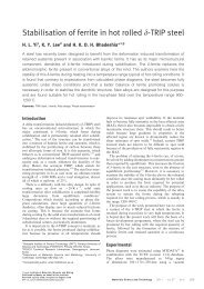
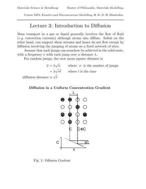
Materials Science & MetallurgyMaster of Philosophy, Materials Modelling,Course MP6, Kinetics and Microstructure Modelling, H. K. D. H. BhadeshiaLecture 3: Introduction to DiffusionMass transport in a gas or liquid generally involves the flow of fluid(e.g. convection currents) although atoms also diffuse. Solids on theother hand, can support shear stresses and hence do not flow except bydiffusion involving the jumping of atoms on a fixed network of sites.Assume that such jumps can somehow be achieved in the solid state,with a frequency ν with each jump over a distance λ.For random jumps, the root mean square distance isx = λ √ ndiffusion distance ∝ √ twhere n is the number of jumps= λ √ νt where t is the timeDiffusion in a Uniform Concentration GradientλCC+δCCxδCFig. 1: Diffusion Gradient

Concentration of solute, C, number m −3Each plane has Cλ atoms m −2 (Fig. 1){ } ∂CδC = λ∂xAtomic flux, J, atoms m −2 s −1J L→R = 1 6 νCλJ R→L = 1 ν(C + δC)λ6Therefore, the net flux along x is given byJ net = − 1 6 ν δC λ= − 1 { } ∂C6 ν λ2 ∂x{ } ∂C≡ −D∂xThis is Fick’s first law where the constant of proportionality is called thediffusion coefficient in m 2 s −1 . Fick’s first law applies to steady state fluxin a uniform concentration gradient. Thus, our equation for the meandiffusion distance can now be expressed in terms of the diffusivity asx = λ √ νt with D = 1 6 νλ2 giving x = √ 6Dt ≃ √ DtNon–Uniform Concentration GradientsSuppose that the concentration gradient is not uniform (Fig. 2).{ } ∂CFlux in = −D∂x1{ } ∂CFlux out = −D∂x2[{ } { ∂C ∂ 2 }]C= −D + δx∂x ∂x 21

unitareaδx1 2CxFig. 2: Non–uniform concentration gradientIn the time interval δt, the concentration changes δCδCδx = (Flux in – Flux out)δt∂C∂t = CD∂2 ∂x 2assuming that the diffusivity is independent of the concentration. Thisis Fick’s second law of diffusion.This is amenable to numerical solutions for the general case butthere are a couple of interesting analytical solutions for particular boundaryconditions. For a case where a fixed quantity of solute is plated ontoa semi–infinite bar (Fig. 3),boundary conditions:C{x, t} =∫ ∞0C{x, t}dx = Band C{x, t = 0} = 0√ B { −x2expπDt 4DtNow imagine that we create the diffusion couple illustrated in Fig. 4,by stacking an infinite set of thin sources on the end of one of the bars.Diffusion can thus be treated by taking a whole set of the exponential}

Carea undereach curve isconstantx∞Fig. 3: Exponential solution. Note how the curvaturechanges with time.functions obtained above, each slightly displaced along the x axis, andsumming (integrating) up their individual effects. The integral is in factthe error functionerf{x} = 2 √ π∫ xso the solution to the diffusion equation is0exp{−u 2 }duboundary conditions:C{x = 0, t} = C sand C{x, t = 0} = C 0{ } xC{x, t} = C s − (C s − C 0 )erf2 √ DtThis solution can be used in many circumstances where the surfaceconcentration is maintained constant, for example in the carburisationor decarburisation processes (the concentration profiles would be thesame as in Fig. 4, but with only one half of the couple illustrated). Thesolutions described here apply also to the diffusion of heat.Mechanism of DiffusionAtoms in the solid–state migrate by jumping into vacancies (Fig. 5).The vacancies may be interstitial or in substitutional sites. There is,

C AC sC Bx∞∞Fig. 4: The error function solution. Notice that the“surface” concentration remains fixed.InterstitialSubstitutionalFig. 5: Mechanism of interstitial and substitutionaldiffusion.nevertheless, a barrier to the motion of the atoms because the motionis associated with a transient distortion of the lattice.Assuming that the atom attempts jumps at a frequency ν 0 , thefrequency of successful jumps is given by}ν = ν 0 exp{− G∗kT{ }}S∗≡ ν 0 exp ×exp{− H∗k kT} {{ }independent of Twhere k and T are the Boltzmann constant and the absolute tempera-

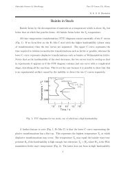
ture respectively, and H ∗ and S ∗ the activation enthalpy and activationentropy respectively. SinceD ∝ ν we find D = D 0 exp{− H∗A plot of the logarithm of D versus 1/T should therefore give a straightline (Fig. 6), the slope of which is −H ∗ /k. Note that H ∗ is frequentlycalled the activation energy for diffusion and is often designated Q.kT}Fig. 6: Typical self–diffusion coefficients for puremetals and for carbon in ferritic iron. The uppermostdiffusivity for each metal is at its melting temperature.The activation enthalpy of diffusion can be separated into two components,one the enthalpy of migration (due to distortions) and the enthalpyof formation of a vacancy in an adjacent site. After all, for theatom to jump it is necessary to have a vacant site; the equilibrium concentrationof vacancies can be very small in solids. Since there are manymore interstitial vacancies, and since most interstitial sites are vacant,interstitial atoms diffuse far more rapidly than substitutional solutes.Kirkendall EffectDiffusion is at first sight difficult to appreciate for the solid state. Anumber of mechanisms have been proposed historically. This includes avariety of ring mechanisms where atoms simply swap positions, but controversyremained because the strain energies associated with such swapsmade the theories uncertain. One possibility is that diffusion occurs by

atoms jumping into vacancies. But the equilibrium concentration of vacanciesis typically 10 −6 , which is very small. The theory was thereforenot generally accepted until an elegant experiment by Smigelskas andKirkendall (Fig. 7).Fig. 7: Diffusion couple with markersThe experiment applies to solids as well as cible liquids. Considera couple made from A and B. If the diffusion fluxes of the two elementsare different (|J A | > |J B |) then there will be a net flow of matter past theinert markers, causing the couple to shift bodily relative to the markers.This can only happen if diffusion is by a vacancy mechanism.An observer located at the markers will see not only a change inconcentration due to intrinsic diffusion, but also because of the Kirkendallflow of matter past the markers. The net effect is described bythe usual Fick’s laws, but with an interdiffusion coefficient D which isa weighted average of the two intrinsic diffusion coefficients:D = X B D A + X A D Bwhere X represents a mole fraction. It is the interdiffusion coefficientthat is measured in most experiments.Structure Sensitive DiffusionCrystals may contain nonequilibrium concentrations of defects suchas vacancies, dislocations and grain boundaries. These may provide easydiffusion paths through an otherwise perfect structure. Thus, the grainboundary diffusion coefficient D gb is expected to be much greater thanthe diffusion coefficient associated with the perfect structure, D P .

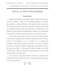
δrFig. 8: Idealised grainAssume a cylindrical grain. On a cross section, the area presentedby a boundary is 2πrδ where δ is the thickness of the boundary. Notethat the boundary is shared between two adjacent grains so the thicknessassociated with one grain is 1 2δ. The ratio of the areas of grain boundaryto grain is thereforeratio of areas = 1 2 × 2πrδπr 2 = δ r = 2δdwhere d is the grain diameter (Fig. 8).For a unit area, the overall flux is the sum of that through thelattice and that through the boundary:so that2δJ ≃ J P + J gbd2δD measured = D P + D gbdNote that although diffusion through the boundary is much faster, thefraction of the sample which is the grain boundary phase is small. Consequently,grain boundary or defect diffusion in general is only of importanceat low temperatures where D P ≪ D gb (Fig. 9).Thermodynamics of diffusionFick’s first law is empirical in that it assumes a proportionalitybetween the diffusion flux and the concentration gradient. However,diffusion occurs so as to minimise the free energy. It should thereforebe driven by a gradient of free energy. But how do we represent thegradient in the free energy of a particular solute?

Dgbln{D}DPD measuredD gb2δd0.7T m1/TFig. 9: Structure sensitive diffusion. The dashed linewill in practice be curved.Diffusion in a Chemical Potential GradientFick’s laws are strictly empirical. Diffusion is driven by gradientsof free energy rather than of chemical concentration:J A = −C A M A∂µ A∂xso thatD A = C A M A∂µ A∂C Awhere the proportionality constant M A is known as the mobility of A.In this equation, the diffusion coefficient is related to the mobility bycomparison with Fick’s first law. The chemical potential is here definedas the free energy per mole of A atoms; it is necessary thereforeto multiply by the concentration C A to obtain the actual free energygradient.The relationship is remarkable: if ∂µ A /∂C A > 0, then the diffusioncoefficient is positive and the chemical potential gradient is along thesame direction as the concentration gradient. However, if ∂µ A /∂C A < 0then the diffusion will occur against a concentration gradient!