R&S®Power Viewer Plus Software Manual - Rohde & Schwarz
R&S®Power Viewer Plus Software Manual - Rohde & Schwarz
R&S®Power Viewer Plus Software Manual - Rohde & Schwarz

Create successful ePaper yourself
Turn your PDF publications into a flip-book with our unique Google optimized e-Paper software.
R&S Power <strong>Viewer</strong> <strong>Plus</strong><strong>Software</strong> <strong>Manual</strong>R&S ® Power <strong>Viewer</strong> <strong>Plus</strong>V 5.6Printed in Germany<strong>Manual</strong> 1
R&S Power <strong>Viewer</strong> <strong>Plus</strong>Contents16.11 Automatic Pulse Measurement .................... 8816.11.1 Measurement Results ..................... 9116.12 Common Measurement Tasks ..................... 9317 Statistics 9417.1 Settings ..................................... 9417.2 Graphical Data View ............................ 9617.3 PDF Mode ................................... 9717.3.1 PDF Background Information ............... 9817.4 CDF Mode .................................. 10017.5 CCDF Mode ................................. 10118 Timeslot Mode 10218.1 Settings .................................... 10218.2 Graphical Data View ........................... 10519 Multi-Channel Power Measurements 10619.1 Channel Configuration .......................... 10719.2 Measurement Settings .......................... 10819.3 Mathematical Expressions ....................... 10920 Script-Based Measurement 11020.1 Script Syntax ................................ 11120.1.1 Variables ............................. 11120.1.2 Predefined Variables ..................... 11120.1.3 Variable Value Assignments ............... 11220.1.4 Equations ............................. 11320.1.5 Comments ............................ 11320.1.6 Suppressing Output ..................... 11320.1.7 Waiting Periods ........................ 11320.1.8 Loops ................................ 11420.1.9 Defining Devices ........................ 11420.1.10 Waiting for Measurement Completion ......... 11520.1.11 SCPI Commands and Queries .............. 11520.1.12 Reading Scalar Results ................... 11620.1.13 Reading Array Results ................... 11620.1.14 Converting Readings ..................... 11720.1.15 Printing to the Log Window ................ 11720.1.16 Displaying Scalar Results ................. 11720.1.17 Displaying Array Data Numerically ........... 11720.1.18 Displaying Array Data as a Bargraph ......... 11820.1.19 Displaying Array Data as a Trace ............ 11820.1.20 Saving Array Data to Text File .............. 11920.1.21 Sending Data to Processing Panels .......... 11920.2 Triggered Average Power Measurement ............. 12020.3 Burst Power Measurement ...................... 12120.4 Buffered-Mode Measurements .................... 12221 Data Processing Panels 12321.1 The Data Log ................................ 12521.1.1 Settings .............................. 12621.1.2 The Context Menu ...................... 12921.1.3 The Time Line Indicator ................... 13021.1.4 Zooming .............................. 13021.2 Limit Monitoring .............................. 131<strong>Manual</strong> 5
R&S Power <strong>Viewer</strong> <strong>Plus</strong>Contents21.2.1 Settings .............................. 13221.2.2 Configuring the Server ................... 13421.2.3 Client Connections ...................... 13621.3 Statistical Analysis ............................ 13721.3.1 Histogram Display ....................... 13821.3.2 Q-Q-Plot ............................. 13921.3.3 The Context Menu ...................... 14021.3.4 Analysis-Panel Settings ................... 14122 Updating the Sensor Firmware 14222.1 Recovering from a Failed Update .................. 14423 Programming Guide 14523.1 Sensor Resource Strings ........................ 14523.2 Numeric Results .............................. 14623.3 Opening and Closing the Sensor Connection ......... 14623.4 Multiple Sensors .............................. 14623.5 Error Handling ............................... 14723.6 Zeroing ..................................... 14723.7 Identifying a Sensor (*IDN?) ...................... 14823.8 Continuous Average Power Measurement ........... 14823.9 Trace Measurements .......................... 15123.9.1 Single-Shot Events ...................... 15323.9.2 Peak Trace Data ........................ 15423.9.3 Automatic Pulse Measurement ............. 15524 Customer Support 15725 Open Source Acknowledgment 15726 Licenses 15826.1 GNU Lesser General Public License (LGPL) 2.1 ....... 158<strong>Manual</strong> 6
R&S Power <strong>Viewer</strong> <strong>Plus</strong>Overview2 OverviewThe new R&S NRP-Z power sensors from <strong>Rohde</strong> & <strong>Schwarz</strong> representthe latest in power measurement technology. They offer all thefunctionality of conventional power meters, and more, within the smallhousing of a power sensor. The USB interface on an R&S NRPZ sensorenables operation with an R&S NRP power meter, or with a PC runningunder either Microsoft ® Windows ® , Mac OS X, or Linux.R&S Power <strong>Viewer</strong> <strong>Plus</strong> is an easy-to-use, feature-packed softwarepackage that offers capabilities beyond those of a regular power meter.It simplifies measurement tasks, such as average-power, timeslot,statistics and trace measurements. In addition, up to four sensors canbe utilized for measuring average power simultaneously. Results, suchas the reflection coefficient or gain, can be computed from themeasured values.Particularly the capabilities for use with a desktop or laptop PC make anR&SNRPZ sensor an ideal and cost-effective solution for lab testing orfor automated systems. The rugged design is suitable for use in thefield for performing such tasks as servicing antenna systems.This manual describes the installation and use of thePower <strong>Viewer</strong> <strong>Plus</strong> software. This application is part of theR&S ® NRP Toolkit and is available free of charge from the<strong>Rohde</strong> & <strong>Schwarz</strong> website.To enable integration of the sensor into custom ATE systems, aversatile and powerful VXI PnP driver is available forMicrosoft ® Windows ® , Mac OS X, and Linux-based systems. Codingexamples can be found at the end of this manual.<strong>Manual</strong> 7
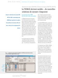
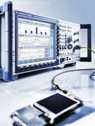
R&S Power <strong>Viewer</strong> <strong>Plus</strong>Key <strong>Software</strong> Features3 Key <strong>Software</strong> FeaturesPower <strong>Viewer</strong> <strong>Plus</strong> is powerful PC software that simplifies manymeasurement tasks. This software is part of the R&S NRP Toolkit andis available free of charge. The following overview lists some of the keyfeatures that Power <strong>Viewer</strong> <strong>Plus</strong> offers.• Measuring the average and peak powers and viewing thenumeric results. Optionally, adding an analog bar display, atrend chart or statistical analysis.Fig. 3.1: Viewing measurement results.• Viewing the RF power envelope down to a resolution of5 ns/div; measuring pulse parameters with automatic pulseanalysis; using markers, and measuring within time gates.Fig. 3.2: Pulse measurement.<strong>Manual</strong> 8
R&S Power <strong>Viewer</strong> <strong>Plus</strong>Key <strong>Software</strong> Features• Performing 4-channel statistical analysis on any measureddata.Fig. 3.7: Four-channel statistical analysis.• Configuring 16-channel limit monitoring for any measured data;optionally, sending limit violations to a remote host via a TCP/IPserver.Fig. 3.8: Limit monitoring.<strong>Manual</strong> 11
R&S Power <strong>Viewer</strong> <strong>Plus</strong>Key <strong>Software</strong> Features• Creating custom measurements in script mode.Fig. 3.9: Script mode for custom measurements.Please note that some of the features listed above are only supportedby certain R&S NRP-Z power sensors. For example, thermal sensorsdo not provide statistical signal analysis or trace measurements.<strong>Manual</strong> 12
R&S Power <strong>Viewer</strong> <strong>Plus</strong>Power Sensor Technologies4 Power Sensor Technologies<strong>Rohde</strong> & <strong>Schwarz</strong> offers a large choice of USB power sensors that usedifferent technologies and cover a wide range of frequencies and powerlevels. This chapter briefly outlines the differences between the sensortechnologies and indicates which sensor would best fit certainmeasurement tasks.All R&S NRPZ power sensors are standalone instruments that containthe detector, the analog circuitry, and the digital signal processing in asingle housing. The entire instrument is fully characterized during theproduction process, which eliminates the need for later calibration usinga reference power source.Zeroing is generally only required for measuring low power levels, inwhich case the zeroing offset, noise, and drift stated in the specificationsheet contribute to the overall accuracy.4.1 Thermal Power SensorsThermal sensors use a load resistor for converting the RF power intoheat. The temperature difference between this resistor and thesurrounding area is measured by thermocouples. The resulting DCvoltage is proportional to the RF power.coaxial RF feederco-planar linethermaltransducer1 mmtaperedtransmisssionFig. 4.1.1: Detector design in thermal power sensor.The <strong>Rohde</strong> & <strong>Schwarz</strong> thermal power sensors can be used from DC upto their specified upper frequency limit. The dynamic range is typically inthe order of 55 dB and starts at power levels of around –35 dBm.Thermal power sensors provide the highest accuracy and linearity of allpower sensors on the market. Their measurements are not influencedby the modulation or harmonics, and the results always represent theaverage signal power.However, the nature of the underlying sensor technology limits thedynamic range. Furthermore, the measurement speed is generallyslower than that of diode sensors. Thermal sensors cannot measure theenvelope of an RF signal.4.2 CW Power SensorsCW sensors are simple diode sensors that contain a half-wave orfull-wave rectifier as the detector element. At power levels below-20 dBm, the diode characteristic provides an almost linear relationshipbetween the detector output voltage and the RF power. This powerrange is referred to as the square-law region of the detector diode.CW sensors typically use the diode at power levels beyond thesquare-law region, and the software must compensate for the resulting<strong>Manual</strong> 13
R&S Power <strong>Viewer</strong> <strong>Plus</strong>Power Sensor TechnologiesFig. 4.5.1: Wideband power sensor design.Similar to CW sensors, the wideband diode sensor's digital signalprocessing circuitry compensates the non-linear diode characteristic inrealtime. Due to the wider bandwidth and fast sampling rate, this is evenpossible for fast amplitude changes (AM) of the RF envelope.Wideband diode sensors are ideal when the RF envelope should bemeasured, e.g. for the analysis of pulsed signals. Additionally, thesedevices can measure the signal statistics, such as the PDF, CDF,CCDF, and average power for modulated signals.The following chart shows the relationship between power levels andapplications that generally fit a wideband diode sensor.Average Power,f mod< BWAv. Power,f mod> BWPeak PowerEnvelope (Averaged)Envelope (Real Time)-60 dBm-20 dBm+23 dBmFig. 4.5.2: Wideband power sensor applications.At power levels below –20 dBm (square-law region), these sensorsexhibit little sensitivity to modulation and harmonics. Average powermeasurements are possible down to a level of about –60 dBm.For higher power levels, care must be taken when the RF envelope isamplitude modulated at frequencies that exceed the detector's analogbandwidth. In such cases, it is no longer possible to compensate the RFenvelope in realtime, and measurement errors in the order of severalpercent may occur.The wider bandwidth used by these sensors generally implies a highernoise floor. Average power measurements overcome this issue byusing averaging techniques. When taking single-shot measurements,however, the higher noise floor must be considered.This is especially the case with peak power measurements. Please seethe chapter 15.4, "Continuous Power Measurements – Accuracy ofPeak Power Measurements" in this document for more details.It must also be noted that triggering is always a realtime process that isbased on samples that have not yet been subject to averaging. As aresult, power levels in the order of –20 dBm or higher are required when<strong>Manual</strong> 15
R&S Power <strong>Viewer</strong> <strong>Plus</strong>Power Sensor Technologiesusing the sensor's internal trigger feature. Decreasing the sensor'sbandwidth decreases the noise floor and, therefore, also decreases thelower trigger-level limit.5 Uncertainty CalculationThis chapter briefly explains how to calculate the measurementuncertainty based on the figures provided in the sensor's specifications.The data sheet lists the absolute uncertainty for power measurementsin dB depending on the power level and frequency. Other contributors,such as zero offset or noise, are provided in watts and can beconverted into dB using the following equation.e=10dB⋅log P P PThis equation uses P as the power level of interest and ΔP as therelative error. The result is the error e in dB.Uncertainties are statistical measures, and they must be added bysumming up the squared uncertainties and then calculating the squareroot:U =U 1 2 U 2 2 U 3 2 This equation can be used for uncertainties in logarithmic scale (dB) orin percent (%).Uncertainties are commonly provided in dB, but the following equationpermits conversion into percent:U %=100%⋅10U dB10 dB −1To gain a simple approximation, the following formula can be used:U %≈10⋅ln 10⋅U dB=23⋅U dB<strong>Manual</strong> 16
R&S Power <strong>Viewer</strong> <strong>Plus</strong>Uncertainty Calculation5.1 Measurements at –10 dBmThe power level range from –10 dBm to 0 dBm is widely used.Therefore, our first example here calculates the absolute uncertainty forthe R&S NRP-Z11 when measuring a CW signal at 2 GHz and at apower level of –10 dBm. The temperature shall be 30 ºC.All values marked with an arrow (►) are taken from the R&S NRPZxxPower Sensor Specifications that are available on the <strong>Rohde</strong> & <strong>Schwarz</strong>website.Power level in W 100 µW► Used path 2► Uncertainty for absolutepower measurements 0.077 dB► Zero Offset 47 nW 0.002 dB► Zero Drift 10 nW 0.0004 dB► Measurement noise6.3 nWMultiplier for 40 ms integrationTime is sqrt(10.24s/T) x 16= 100.8 nW 0.004 dBTotal expanded uncertainty 0.077 dB1.79 %The example shows that the influence of zero offset and drift isnegligible. Consequently, zeroing of the sensor is not required whenperforming practical measurement tasks. The integration time can beset to a very short value of 40 ms. This means that an averaging countof one, combined with two chopper cycles and a measurement window(aperture) of 20 ms, is sufficient.The total integration time is twice the aperture time multiplied by theaveraging filter count.<strong>Manual</strong> 17
R&S Power <strong>Viewer</strong> <strong>Plus</strong>Uncertainty Calculation5.2 Measurements at –50 dBmThis example calculates the absolute uncertainty for the R&S NRPZ11when used for measuring a CW signal at 2 GHz and at a very lowpower level of –50 dBm. The temperature shall be 30 ºC.All values marked with an arrow (►) are taken from the R&S NRPZxxPower Sensor Specifications that are available from the<strong>Rohde</strong> & <strong>Schwarz</strong> website.Power level in W10 nW► Used path 1► Uncertainty for absolutepower measurements 0.081 dB► Zero offset after zeroing 104 pW 0.045 dB► Zero drift after zeroing 35 pW 0.0015 dB► Measurement noise65 pWMultiplier for 1.28 s integrationtime is sqrt(10.24s/T) x 2.8= 182 pW 0.078 dBTotal expanded uncertainty 0.12 dB2.8 %After zeroing, the absolute accuracy is 0.12 dB when using anintegration time of 1.28 s. This integration time can be achieved with anaverage filter count of 32 and a measurement window of 20 ms. Furtherimprovement of the uncertainty is possible by increasing the averagingfilter count.The total integration time is twice the aperture time multiplied by theaveraging filter count.<strong>Manual</strong> 18
R&S Power <strong>Viewer</strong> <strong>Plus</strong>Uncertainty Calculation5.3 The Influence of MismatchPower sensors are always calibrated to measure the power of theincident RF wave. This means that the sensor corrects the reading forthe internal losses and reflections. As a result, different power sensorsthat were connected to an ideal 50 ohm source would all show exactlythe same result.In the real world, however, neither the power sensor nor the sourcematch an impedance of 50 ohms exactly. The reflection that is causedby the power sensor itself is specified by the standing wave ratio(SWR), which is typically around 1.2. This means that a small portion ofthe RF wave is reflected back towards the source as a return wave. Anideal source would absorb this return wave entirely. Since the powersensor is calibrated to measure the incident wave and compensates forits own reflections, the reading is correct.Real signal sources are not ideal either. They also reflect a portion ofthe return wave back to the power sensor. This portion adds to theincident RF wave and influences the measurement result.The uncertainty calculations in the previous chapter did not include theerror caused by mismatch. The following equation shows the minimumand maximum possible incident power based on the reflectioncoefficient of the source and the load:P GZ0P GZ01r G r L 2P i1−r G r L 2P GZ0: Power from signal sourceP i: Incident power to powersensorr G: Generator reflectioncoefficientr L: Load reflection coefficientDepending on the phase angle, the incident power varies between theleft and right term of the equation. The following equations canapproximate the maximum relative deviation ε max between the sourcepower P GZ0 and the incident power P i: max%≈200 % r Gr Lfor max20% maxdB≈8.7dB r Gr Lfor max1dBUncertainty calculations use statistical figures instead of the ε max errorsfrom the equations above. The following equation shows therelationship between the expanded uncertainty (k = 2) and the error.U dB=2⋅ max dB2This shows that the expanded uncertainty used for the uncertaintycalculation is higher than the maximum error.<strong>Manual</strong> 19
R&S Power <strong>Viewer</strong> <strong>Plus</strong>Uncertainty CalculationData sheets often express the impedance matching of a device as astanding wave ratio (SWR). The relationship between the SWR and thereflection coefficient is expressed by the following equations:s= 1r L1−r Lr L= s−1s1The example below demonstrates the influence of mismatch caused bya signal source that is directly connected to a power sensor:Load: R&S NRPZ11 SWR = 1.2 r L = 0.09Source: R&S SMBV100A SWR = 1.6 r G = 0.23U dB = 2 · 0.707 · ± 8.7 dB · 0.09 · 0.23 = ± 0.25 dB<strong>Manual</strong> 20
R&S Power <strong>Viewer</strong> <strong>Plus</strong><strong>Software</strong> Installation6 <strong>Software</strong> InstallationThe following section outlines the process for installingPower <strong>Viewer</strong> <strong>Plus</strong> on various platforms.6.1 System RequirementsIf the sensors are to be controlled by a PC rather than by using theR&S NRP base unit, certain prerequisites must be fulfilled.Hardware requirements• Desktop PC or laptop, or an Intel-based Apple Mac• Keyboard and mouse• 800 x 600 screen resolution (1024 x 768 recommended)• USB 1.1 or 2.0 interface• Multi-TT based USB hub architecture recommended• R&S NRP-Z3, R&S NRP-Z4, or R&S NRP-Z5 adapterOperating systems (choice of)• Microsoft ® Windows ® XP 32-Bit• Microsoft ® Windows ® 7 32/64-Bit• Mac OS X• 32-Bit Linux distribution with kernel ≥ 2.6.x(e.g. Ubuntu 10.4 LTS x86, 11.4 x86)R&S software packages• R&S NRP Toolkit. It provides the required USB drivers.• The Power <strong>Viewer</strong> <strong>Plus</strong> software is supplied with the R&S NRPToolkit.<strong>Manual</strong> 21
R&S Power <strong>Viewer</strong> <strong>Plus</strong><strong>Software</strong> Installation6.2 Installation on Windows-Based SystemsThe application is part of the R&S NRP Toolkit. This toolkit contains allrequired USB drivers, as well as toolkit applications andPower <strong>Viewer</strong> <strong>Plus</strong>.1. Disconnect all NRP-Zxx power sensors from the PC.2. Start the R&S NRP Toolkit installer and follow the instructions.3. In the Choose Components window, you must enable the USBdrivers if the toolkit has never been installed before. If aprevious R&S NRP Toolkit installation is found, the installermay offer an option to update the drivers. It is highlyrecommended that you enable the USB driver update.4. Enable R&S NRP Toolkit if you need additional toolkitprograms, such as the S-parameter update, or the classicPower <strong>Viewer</strong>.5. Enable R&S Power <strong>Viewer</strong> <strong>Plus</strong>.Fig. 6.2.1: R&S NRP Toolkit installer.After the installation has completed, the sensors can be connected tothe PC. If the USB drivers were updated or newly installed, recognizingthe sensor may take more time when it is plugged in for the very firsttime.<strong>Manual</strong> 22
R&S Power <strong>Viewer</strong> <strong>Plus</strong><strong>Software</strong> Installation6.3 Installation on Linux-Based SystemsThis application is part of the R&S NRP Toolkit. In contrast to theWindows R&S NRP Toolkit, the Linux version contains the followingcomponents:• NrpZ Kernel module• NrpLib Low-level driver• RsNrpZ VXI PnP driver• HTML help files for the VXI PnP driver• Power <strong>Viewer</strong> <strong>Plus</strong> and PDF manual• Example programs for use with VXI PnP driverThe toolkit comes as a self-extracting archive that must be run with rootuser permissions:# sudo ./NrpLinuxPckg_.runRunning the installer requires the following tools and packages to bepresent in the system:• dialog, base64, tar, gcc• ia32-libs (on amd64 systems only)• Kernel modules under /lib/modules/• Kernel headers under /usr/include/linuxThe self-extracting archive first extracts it's content to a temporarydirectory under /tmp and then transfers control to the installation scriptin this directory.Fig. 6.3.1: R&S NRP Toolkit installer for Linux.If the basic system requirements are met, the screen shown aboveshould appear and prompt the user to confirm if the installation shouldstart.Next, the legal terms are displayed. Use q to quit this screen, and thenaccept the license terms.<strong>Manual</strong> 23
R&S Power <strong>Viewer</strong> <strong>Plus</strong><strong>Software</strong> Installation6.5 Sensor Firmware RequirementsPower <strong>Viewer</strong> <strong>Plus</strong> may require newer firmware versions on certainpower sensors. Please see the firmware update section in this manualfor more details on updating the sensor firmware. The latest firmwarefiles are available free of charge from the <strong>Rohde</strong> & <strong>Schwarz</strong> website.R&S NRP-Z8xR&S NRP-Z1xR&S NRP-Z2xR&S NRP-Z3xR&S NRP-Z5x1.16 or later (1.20 recommended)4.08 or later4.08 or later4.08 or later4.08 or later<strong>Manual</strong> 28
R&S Power <strong>Viewer</strong> <strong>Plus</strong><strong>Software</strong> Installation6.6 Supported R&S NRPZ SensorsThe following table provides an overview of the sensors that aresupported in Power <strong>Viewer</strong> <strong>Plus</strong>.SensorUSBIDSupported MeasurementCont Trace Timeslot StatisticsNRP-Z11 0x0C ● ● ●NRP-Z21 0x03 ● ● ●NRP-Z211 0xA6 ● ● ●NRP-Z22 0x13 ● ● ●NRP-Z221 0xA7 ● ● ●NRP-Z23 0x14 ● ● ●NRP-Z24 0x15 ● ● ●NRP-Z31 0x2C ● ● ●NRP-Z41 0x96 ● ● ●NRP-Z51 0x16 ●NRP-Z52 0x17 ●NRP-Z55 0x18 ●NRP-Z56 0x19 ●NRP-Z57 0x70 ●NRP-Z58 0xA8 ●NRP-Z91 0x21 ●NRP-Z81 0x23 ● ● ● ●NRP-Z85 0x83 ● ● ● ●NRP-Z86 0x95 ● ● ● ●NRP-Z27 0x2F ●NRP-Z28 0x51 ● ● ●NRP-Z37 0x2D ●NRP-Z92 0x62 ●NRP-Z98 0x52 ●NRPC33 0xB6 ●NRPC40 0x8F ●NRPC50 0x90 ●NRPC33-B1 0xC2 ●NRPC40-B1 0xC3 ●NRPC50-B1 0xC4 ●FSH-Z1 0x0B ●FSH-Z18 0x1A ●If no sensor is detected, Power <strong>Viewer</strong> <strong>Plus</strong> automatically activates asimulated sensor called NRP-Z00.The vendor ID for all R&S NRP-Zxx sensors is 0x0AAD.<strong>Manual</strong> 29
R&S Power <strong>Viewer</strong> <strong>Plus</strong><strong>Software</strong> Installation6.7 Running Multiple InstancesOnly one instance of Power <strong>Viewer</strong> <strong>Plus</strong> can be run at a time. Thislimitation is required, because the low-level drivers do not supportsimultaneous access to the sensors from multiple applications.Power <strong>Viewer</strong> <strong>Plus</strong> checks to see if any other instance is alreadyrunning on the system. If so, a warning message appears.Fig. 6.7.1: Warning message indicating that an application is alreadyrunning.Power <strong>Viewer</strong> <strong>Plus</strong> does not detect if any other application is alreadyaccessing the low-level drivers. For this reason, it is advisable to closeall other R&S NRP-Z-related applications before startingPower <strong>Viewer</strong> <strong>Plus</strong>.<strong>Manual</strong> 30
R&S Power <strong>Viewer</strong> <strong>Plus</strong>Command Line Options7 Command Line Options7.1 General OptionsThe Power <strong>Viewer</strong> <strong>Plus</strong> software supports a set of command lineoptions that affect the application's look and feel as well its startupbehavior:--nativeThe user interface look is left as native as possible.--classic-pvThis option starts Power <strong>Viewer</strong> <strong>Plus</strong> in a mode in which it only displaysthe continuous power measurement window. This is similar to theclassic Power <strong>Viewer</strong> application:• Disables all features but the continuous power measurement.• Always starts with a fixed application window size.• Continuous power measurement is activated.• The analog bar and trend display are not available.• The measurement starts automatically if a sensor is detected.--no-splashThis option omits the initial splash screen and speeds up the applicationstartup.--project This option loads a specific project file at startup. If the application isavailable, the default project file is written. If the specified project file isnot available, the default settings are applied.--sensor This option includes –no-splash and omits the initial sensor scanning.Instead, the specified sensor is made available regardless of itsphysical availability. The sensor must be defined by the sensor type andby its serial number (for example: “Z11,123456”).--no-multiDisables the multi-channel measurement mode.<strong>Manual</strong> 31
R&S Power <strong>Viewer</strong> <strong>Plus</strong>Command Line Options--no-flashDisables the firmware flash dialog.--no-timeslotDisables the timeslot measurement mode.--no-statisticsDisables the statistics measurement mode.--no-traceDisables the trace measurement mode.--no-scriptingDisables the scripting measurement mode.--no-datalogDisables the data log window.--no-analysisDisables the data analysis window.--no-monitorDisables the limit monitoring window.--debugWrites additional log messages to the message log window. This maybe useful for debugging software problems.<strong>Manual</strong> 32
R&S Power <strong>Viewer</strong> <strong>Plus</strong>Command Line Options7.2 Setting the Application StyleThe style of the Power <strong>Viewer</strong> <strong>Plus</strong> user interface can be changed usingthe -style command-line option. Changing the style might be useful ifthe application should use the operating system's look and feel. Bydefault, Power <strong>Viewer</strong> <strong>Plus</strong> uses an internal style that is independent ofthe underlying operating system.-style User Interface ExamplePlastiqueCleanlooksWindowsMotifWindowsXP<strong>Manual</strong> 33
R&S Power <strong>Viewer</strong> <strong>Plus</strong>Connecting Sensors to the PC8 Connecting Sensors to the PCPlease see your R&S NRP-Z power sensor's manual for information onhow to put the sensor into operation. Follow these instructions toprevent damage to the sensor, particularly if you are putting it intooperation for the first time.The following section provides additional information that is related tothe USB interface or to operating multiple sensors simultaneously.8.1 Using Multiple SensorsIf multiple sensors need to be connected to a single computer, check toensure that the overall current requirements for operating all sensorscan be met. Each single sensor draws between 300 mA and 500 mA,depending on the sensor type.Example:The R&S NRP-Z81 sensor is rated at up to 500 mA supply current.Using four sensors simultaneously on one hub requires a total currentof at least two amperes. Many consumer hubs cannot provide thiscurrent over a long period of time, even if they are rated for this value.For industrial-grade applications, it is advisable to use USB hubs for aDIN rail mount that can provide up to one ampere per USB port and runoff a 24 V power supply. These two manufacturers provide suchdevices:• Beckhoff ( www.beckhoff.com ) CU8005• Lütze ( www.luetze.de ) 745581 DIOHUB USB 4Other industrial or office-type hubs that have shown good performanceat the time of writing (2009) are:• BELKIN ® Hi-Speed USB 2.0 7-Port Hub F5U237eaAPL-S• Digi ® Hubport/4c or Hubport/7cThe following hub specifications are crucial when multiple powersensors shall be connected to the hub:• Multi-TT switched architecture• Individual port power management, 500 mA per channel<strong>Manual</strong> 34
R&S Power <strong>Viewer</strong> <strong>Plus</strong>Connecting Sensors to the PC8.2 Using USB Extension Hardware8.2.1 R&S NRP-Z3 Active USB AdapterThe figure shows the configuration with the R&S NRP-Z3 active USBadapter, which also makes it possible to feed in a trigger signal for thetimeslot and trace modes. The order in which the cables are connectedis not critical.Fig. 8.2.1: Configuration with the active USB adapter.8.2.2 R&S NRP-Z4 Passive USB AdapterThe figure below is a schematic of the measurement setup. The orderin which the cables are connected is not critical.Fig. 8.2.2: Configuration with the passive USB adapter<strong>Manual</strong> 35
R&S Power <strong>Viewer</strong> <strong>Plus</strong>Connecting Sensors to the PC8.2.3 R&S NRP-Z5 Sensor HubThe R&S NRP-Z5 sensor hub allows up to four power sensors to beoperated on one PC. It combines the following functions:• 4-port USB 2.0 hub with Multi-TT architecture• Power supply• Through-wired trigger bus• Trigger input and trigger output via BNC socketsIt is possible to cascade several R&S NRP-Z5 sensor hubs byconnecting the R&S Instrument port of an R&S NRP-Z5 to one of thesensor ports of another R&S NRP-Z5. However, external triggering andthe use of the Trigger Master function are then not possible. Instead, itis recommended that you connect all R&S NRP-Z5 hubs individually tothe USB host or to an interposed USB hub. Then feed the externaltrigger signal to all R&S NRP-Z5 hubs via their trigger inputs.Fig. 8.2.3: Connecting the USB hub.<strong>Manual</strong> 36
R&S Power <strong>Viewer</strong> <strong>Plus</strong>Connecting Sensors to the PC8.2.4 Third-Party ProductsThis section lists devices that are manufactured by other vendors andhave been used successfully with R&S NRP-Zxx power sensors.<strong>Rohde</strong> & <strong>Schwarz</strong> cannot provide a continuous guarantee that theseproducts will work with R&S NRP-Zxx sensors, because technicalchanges or newer versions of these products are not retested:Icron (www.icron.com) offers the USB Ranger 110/410 products thatare compliant with the USB 1.1 specification and can be used to cover adistance of up to 100 meters by using standard Cat 5 UTP cabling.Icron (www.icron.com) offers the USB Ranger 2224 product that iscompliant with the USB 2.0 specification and can be used to cover adistance of up to 500 meters by using a multi-mode optical fiber.When large distances between the control PC and the sensor(s) arerequired, a combination of the USB Ranger 2224 and the R&S NRP-Z5has demonstrated reliable operation.Fig. 8.2.4: Setup with 100 m optical fibre.Digi (www.digi.com) makes the AnywhereUSB ® Network-enabled USBhub. This product is used to access a USB device over a TCP/IPnetwork.<strong>Manual</strong> 37
R&S Power <strong>Viewer</strong> <strong>Plus</strong>Configuring the Application9 Configuring the ApplicationPower <strong>Viewer</strong> <strong>Plus</strong> provides a settings dialog that can be accessed byselecting Configure → Options from the main menu.This dialog box is structured using separate tabs for drawingoperations, timeouts, hardcopies, USB, and debugging.9.1 Drawing PerformanceThe drawing performance can be adjusted to accommodate slow PCs.Activating these features lowers CPU load or adds additional idle time.Fig. 9.1.1: Drawing performance settings.Disable Transparency EffectsLowers CPU consumption by avoiding semi-transparent drawingoperations. Transparent drawing is used, for example, for the grid linesin the trace mode, because it makes it possible to see trace points thatfall exactly onto a grid line.Number of Video Points for TracesSet to 500 by default, this number provides a good compromisebetween measurement speed and resolution. The higher the number ofvideo points, the higher the CPU load and acquisition time. On lowperformancePCs, it may be desirable to lower this number.<strong>Manual</strong> 38
R&S Power <strong>Viewer</strong> <strong>Plus</strong>Configuring the ApplicationSet Additional Video Update TimeAdds idle time between two measurements. This reduces CPU load andprovides resources to other applications. The default idle time betweentwo measurements is in the order of 100 ms.Disable LCD BackgroundReplaces the blue color gradient used in all LCD displays with a simplegray color. This option is useful for increasing the display contrast andfor reducing CPU usage.Disable Trace Anti-AliasingTurns off anti-aliasing in all trace and statistics measurement panels.Turning anti-aliasing off speeds up drawing operations and reducesCPU usage.<strong>Manual</strong> 39
R&S Power <strong>Viewer</strong> <strong>Plus</strong>Configuring the Application9.2 Hardcopy SettingsPower <strong>Viewer</strong> <strong>Plus</strong> creates print reports or copies measurement resultsto the system clipboard. This greatly simplifies documentation tasks.Please see the "Hardcopy Features" and "Copy to Clipboard" sectionsfor additional details.Fig. 9.2.1: Hardcopy settings.Do Not Invert ColorsBy default, the application uses printer-friendly colors when copyingdata to the system clipboard. This feature can be turned off by choosingnot to invert the screen colors.Use Custom Size...The Copy to Clipboard function always creates a bitmap of a fixed size.This simplifies documentation tasks, since any display resolution maybe used, and you do not need to specifically rescale captured images.<strong>Manual</strong> 40
R&S Power <strong>Viewer</strong> <strong>Plus</strong>Configuring the Application9.3 Timeout-Related SettingsThe Timeout tab is shown below and is mainly used for connectionsacross USB extenders or USB-to-LAN interfaces. These devices oftenintroduce large turnaround times that need to be taken care of.Fig. 9.3.1: Timeout settings.USB CommunicationBy default, this value is set internally to 5 seconds. Connections acrossthe Internet (e.g. using the Digi AnywhereUSB ® device, www.digi.com)may require values of up to 15 seconds.Measurement TimeoutThis function is used internally to set the time between the point when ameasurement is initiated and the maximum waiting time for the result.Normally, the internal time of 5 seconds should be sufficient. However,very slow connections may make it necessary to increase this time.<strong>Manual</strong> 41
R&S Power <strong>Viewer</strong> <strong>Plus</strong>Configuring the Application9.4 USB-Related SettingsThe USB tab is shown below and is used for altering USB interfacerelated settings on Microsoft Windows-based operating systems.Fig. 9.4.1: USB settings.Long Distance ModeThis mode is only available for Windows-based operating systems. Itreduces the number of simultaneous read processes, which lowersUSB resource allocation in the operation systems dramatically.AnywhereUSB ® connections, for example, require activation of the LongDistance Connection mode.Selective Suspend ModeWindows can turn off unused USB hubs or unused ports on USB hubs.This is the default setting on most fresh installations. In some situationsthis mechanism does not work properly and can leave a hub turned offor in an undefined state. Disabling selective suspend turns this powersaving mechanism off for all hubs and subsequently requires a systemreboot. The selective suspend should only be turned off if USB devicesdo not get activated after they were plugged into a USB port.<strong>Manual</strong> 42
R&S Power <strong>Viewer</strong> <strong>Plus</strong>Configuring the Application9.5 USB Device TreeThe Sensors tab is shown below and is used for analyzing the USBdevice tree on Microsoft Windows-based operating systems. The tree ismainly intended for diagnostic purposes because some sensor / hubconfigurations have shown poor performance. These configurations arehighlighted with a yellow exclamation mark.Fig. 9.5.1: USB device tree.The following USB configurations should be avoided:• NRP-Z sensors that are directly connected to Single-TT USBhubs.• NRP-Z sensors that are directly connected to bus powered USBhubs.• NRP-Z sensors that are directly connected to the PC's USBport (root hub).<strong>Rohde</strong> & <strong>Schwarz</strong> generally recommends to operate NRP-Z powersensors with Multi-TT USB hubs. The hub should be equipped with apower supply that is rated for the total current of all connected sensors.Each individual hub port should be capable of delivering up to 500 mAto the USB device.<strong>Manual</strong> 43
R&S Power <strong>Viewer</strong> <strong>Plus</strong>Configuring the Application9.6 Debug OptionsThe debug options are mainly intended for debugging purposes. Thefollowing list contains debug options that may be used with certainmeasurements:contav.fastmode=1multi.fastmode=1This option increases the measurement rate in the continuous power ormulti-channel measurement mode and is explained in more detail in therelated section in this manual.trace.thick=1This option draws bold traces in the trace measurement instead ofusing thin lines. Combined with a low trace point count, this setting isuseful for outdoor service applications.trace.meastime=1When this option is enabled, the Power <strong>Viewer</strong> software displays thetotal trace measurement time in the trace window. This time is theperiod starting at the initiation of the measurement and ending when alldata is received by the host.tsl.peak=0When this setting is disabled, the Power <strong>Viewer</strong> software omits peakreadings in the timeslot measurement mode. Please note that peakmeasurements are subject to higher noise content, and the readingsare only useful for levels greater than –5 dBm.contav.cmd=trace.cmd=multi.cmd=If set accordingly, Power <strong>Viewer</strong> <strong>Plus</strong> appends the SCPI commandsprovided in the command list at the end of themeasurement configuration. The command list can either be a singleSCPI command or a list of commands separated by a semicolon (;).For the multi-channel measurement mode, the channel number mustalso be provided.Using these commands is risky, because it may leave the sensor anduser interface in different states.trace.noinfo=1This option suppresses the Measure information box in the tracewindow.<strong>Manual</strong> 44
R&S Power <strong>Viewer</strong> <strong>Plus</strong>Setting the Application Colors10 Setting the Application ColorsPower <strong>Viewer</strong> <strong>Plus</strong> provides a color settings dialog box that can beaccessed by selecting Configure → Colors from the main menu.All color changes are applied immediately in all application windows.Therefore, it is possible to open windows, such as the tracemeasurement, and observe the color changes directly.Fig. 10.1: Color settings dialog box.PresetThe entire application can be set to one of the predefined colorschemes or to a user-defined color set.Save As…This button saves the user color scheme to a file.Load…This button loads a color scheme from a file and replaces the currentuser color set.<strong>Manual</strong> 45
R&S Power <strong>Viewer</strong> <strong>Plus</strong>Setting the Application ColorsBrightnessThe brightness control changes the brightness for the entire application.Changing the brightness setting does not affect any of the user's colordefinitions.ContrastThe contrast control changes the contrast setting for the entireapplication. Increasing the contrast reduces the brightness ofbackground colors and increases the brightness of foreground colors.Changing the contrast does not affect any of the user's color definitions.Color tilesThe small colored tiles represent the color of the individual elements.One of these tiles can be selected for editing using the HSV colorcontrols.HSV color controlThe application uses the HSV color model to define the applicationcolors. This color model uses hue, saturation and value instead of red,green and blue components.The hue represents the angle on the color wheel between 0° and 360°.This value is meaningless for non-chromatic colors, such as gray. Thesaturation is set in the range between 0 and 255; it defines how strongthe color is. Grayish colors have very low saturation, whereas strongcolors use high saturation values. The value defines the lightness; thisparameter is also set between 0 and 255. The brighter the color is, thehigher the value is.<strong>Manual</strong> 46
R&S Power <strong>Viewer</strong> <strong>Plus</strong>First Steps11 First StepsThe main application window is divided into three major sections.• The measurement window area• The settings panel on the right side• The upper and lower toolbarsOnly one measurement can be active at a time, but it is possible to tilemultiple measurement windows and switch from one to the other. Allmeasurement windows have the same sensor assigned.If the settings panel is enabled, it is always located on the right side. Itscontent changes with the currently activated measurement window.Measurement windowMeasurement-related settingsMeasurement selectionSensor selectionData log running indicatorMeasurement running indicatorGeneralparametersFig. 11.1: The main application window.<strong>Manual</strong> 47
R&S Power <strong>Viewer</strong> <strong>Plus</strong>First Steps11.1 Numeric Entry FieldsThe Power <strong>Viewer</strong> <strong>Software</strong> uses custom entry fields for most numericdata. These entry fields are closely related to regular text entry boxesthat allow the user to enter any text. Custom entry fields differ fromregular entry fields in that they format and validate the user input whenthe enter button is pressed, or the field looses the focus.During the editing process, the entry field changes its background color.That change informs the user that the current data has not yet beenaccepted.Fig. 11.1.1: Custom data entry field after (left) and during (right) editing.Numbers are entered with or without their unit. The unit can be one ofthe following letters:GMkmnupfGigaMegakilomillinanomicropicofemtoThe entry fields also provide a "tooltip" help function that shows theminimum and maximum permissible input value. Additionally, a stepsize can be defined to increase or decrease the value when the mousewheel is turned.Fig. 11.1.2 Example of the help tooltip function.The step value can be defined as follows: First place the cursor in frontof the digit that should serve as the step size. Then press the rightmouse key and select “Set Step from Csr” in the context menu.<strong>Manual</strong> 48
R&S Power <strong>Viewer</strong> <strong>Plus</strong>First Steps11.2 The Menu Bar11.2.1 FileFig. 11.2.1: File settings.File → Load ProjectLoads a previously saved configuration. These settings affect allmeasurements and fully restore the state of the entire application,including window positions.File → Save Project AsSaves the configuration of the entire application to a file. This file maylater be used to restore a measurement configuration. Measurementdata is not saved as part of the settings file.File → ExitAborts all running measurements, disconnects from the power sensor,and subsequently ends the application.11.2.2 SensorFig. 11.2.2: Sensor menu.Sensor → ZeroStarts the zeroing sequence for the selected sensor. For this purpose,the RF signal must be switched off, or the sensor must be disconnectedfrom the signal source. The sensor automatically detects the presenceof any significant power, which causes zeroing to be aborted followedby output of an error message.<strong>Manual</strong> 49
R&S Power <strong>Viewer</strong> <strong>Plus</strong>First StepsThe zeroing process may take more then 8 seconds to complete andvaries with the sensor model.Generally, it is possible to run the sensor zeroing with a small signal(such as broadband noise) applied to the sensor. This makes it possibleto compensate for this signal in later measurements.Sensor → PropertiesDisplays a panel that contains a set of important sensor properties,such as the frequency and power range, as well as the firmwareversion.Sensor → Query Extended InformationReads all available information from the selected sensor. This menuoption is only available when no measurements are running.Sensor → Run Self TestPerforms a self-test on the selected sensor and returns the results astext message. The detector's noise level is measured as part of thesensor self-test routines. This only works when no RF signal is appliedto the sensor's input while the test is running.Sensor → Scan for SensorsStarts the process of detecting available R&S NR-Z USB sensors.Activating this menu item repopulates the sensor selection control. If nosensor is detected, a sensor simulation function (R&S NRP-Z00) will beavailable.Scanning is also performed automatically when new sensors areconnected to the PC or sensors are removed. The automatic scanningcapabilities are inhibited while measurements are running, and theyresume after all measurements have been stopped.Sensor → Channel AssignmentDisplays a panel that allows the user to assign alias names to eachsensor. This simplifies working with multiple sensors. Alias names areonly valid within Power <strong>Viewer</strong> <strong>Plus</strong>.Sensor → Update FirmwareOpens the sensor firmware update dialog. Please see the firmwareupdate section for detailed information about the update process.<strong>Manual</strong> 50
R&S Power <strong>Viewer</strong> <strong>Plus</strong>First Steps11.2.3 MeasurementFig. 11.2.3: Measurement menu.Measurement → StartStarts the measurement in the window that is currently active. Thisbutton is disabled when another measurement window is alreadyrunning. Please note that some sensors may not support allmeasurement modes. In such cases, the start button is disabled, even ifthe measurement window is open and no measurement is running.Measurement → StopStops the currently active measurement. To add a level of protection, ameasurement can only be stopped when its window is active andselected. This prevents unintentional stopping of a measurement.Measurement → ContinuousOpens the panel for the continuous measurement mode. In this mode,the power sensors perform asynchronous measurements on the signalpower over a definable time interval (aperture time).Measurement → TraceOpens the panel for the Trace measurement mode. The panel displaysthe envelope power versus time.Measurement → StatisticsOpens the panel for the Statistics measurement mode. In this mode,the signals CDF, CCDF, or PDF can be measured.Measurement → TimeslotOpens the panel for the Timeslot measurement mode. This modemeasures the average and peak power of a definable number ofsuccessive timeslots.Measurement → Multi ChannelOpens a panel that can display continuous power readings for up to 16sensors.Measurement → ScriptingOpens the scripting window. The scripting measurement module isused to execute SCPI scripts or to define custom measurements.Please see the scripting section for additional details.<strong>Manual</strong> 51
R&S Power <strong>Viewer</strong> <strong>Plus</strong>First Steps11.2.4 Data ProcessingFig. 11.2.4: Data Processing menu.This menu contains functions that do not perform measurements butreceive measured values for evaluation. Most data processing functionsmust be started manually after the measurement has begun. Typically,the data processing automatically finishes when the measurementstops.Data Processing → Data LogThe data log captures up to four different values over a definableperiod. The data is captured in two ways: The default method stores thereadings in up to 20000 data bins (memory). This data can be viewedand exported to a file. The second method writes the captured valuesdirectly to a file while the measurement is running. There is no limitationon the number of data points when writing to a file.Data Processing → AnalysisThe analysis window evaluates up to four measurands statistically. Inthe default configuration, the Power <strong>Viewer</strong> <strong>Plus</strong> creates a histogramview in each analysis channel.Data Processing → Limit MonitorThe limit monitor module compares up to 16 measurands against upperand lower warning and error limits. It can send limit violations to aremote host via its internal TCP/IP server.<strong>Manual</strong> 52
R&S Power <strong>Viewer</strong> <strong>Plus</strong>First Steps11.2.5 WindowFig.11.2.5: Window menu.Window → Copy Graphics to ClipboardSends the content of the currently activated measurement window tothe system clipboard. This option is only available for measurementsthat display their results in graphical form (such as trace, statistics,timeslot and data log measurements). The copy-to-clipboard functionsimplifies documentation tasks, because the graphics can simply bepasted into other applications.Please see chapter 12.2 "Copy to Clipboard" for a detailed description.Window → Save Graphics to FileThis function is similar to the above menu option, but it creates a .pngfile on the user's desktop that contains the screen shot.Window → Print ReportCreates a printout of the measurement that is currently activated. Theprintout is a one-page document that contains the measurement and allimportant sensor settings. Colors are inverted where necessary to avoida black background. This option is only available for measurements thatdisplay their result as graphics (such as trace, statistics, timeslot, anddata log measurements).Please see chapter 12.1 "Print Report" for additional details.Window → Save Measurement DataSaves measurement data from the currently active window to a .csv file.This extension stands for comma-separated values. Files in this formatlist data in columns that are separated by a single comma. This optionis only available for measurements such as the trace, statistics or datalog measurements. Comma-separated value lists can easily beimported into most applications, such as Microsoft ® Excel ® or OpenOffice.Window → Show Tool BarEnables or disables the upper tool bar. Disabling the tool bar is useful ifthe application shall be used with screen resolutions of 800 x 600 pixelsor less.Window → Toggle Settings PanelEnables or disables the settings panel on the right side of theapplication window. Removing the settings panel frees some display<strong>Manual</strong> 53
R&S Power <strong>Viewer</strong> <strong>Plus</strong>First Stepsspace and can be useful if the screen resolution is limited, e.g. 640x480pixels.11.2.6 HelpFig. 11.2.6: Help menu option.Help → About This <strong>Software</strong>Displays program information, such as the software version numberand licensing information.<strong>Manual</strong> 54
R&S Power <strong>Viewer</strong> <strong>Plus</strong>First Steps11.3 The ToolbarThe application provides a main toolbar that is located at the top of themain program window. This toolbar hosts shortcuts to commonly usedfunctions and measurements.Stop measurementStart measurementZero sensorToggle settingsSave measurement dataCopy graphics to clipboardPrint measurement reportSave project fileLoad project fileSave graphics to fileFig. 11.3.1: The main toolbar.11.4 Selecting a SensorA second toolbar is located at the lower border. It is used for sensorselection and for general settings. This toolbar is divided into twosections: The left side provides measurement and data-log runningindicators as well as a control for sensor selection. If no sensor wasdetected during the last USB bus scan, only the sensor simulationfunction (NRP-Z00) is available. This simulation capability can be usedfor basic demonstration and testing of the program's functionality.Fig. 11.4.1: Second toolbar with sensor selection.The application remembers the last sensor selection and tries to reusethis device if it was detected during a USB scan. If the last sensor thatwas used is no longer detected, the first detected sensor is usedinstead.Please note that changing the sensor type may affect measurementsettings. Power <strong>Viewer</strong> <strong>Plus</strong> double-checks measurement settingsbefore a measurement is started and corrects values if necessary.<strong>Manual</strong> 55
R&S Power <strong>Viewer</strong> <strong>Plus</strong>First Steps11.5 General Measurement SettingsThe right toolbar section provides general settings for defining thesignal frequency, level offset, or gamma correction settings, or forselecting the use of an S-parameter set.Fig. 11.5.1: Second toolbar with general settings.Please note that the general settings are applicable to all measurementfunctions, except for multi-channel measurements. The multi-channelmeasurement function provides individual settings for each sensor.Signal FrequencyThis frequency is used to correct measurement results in various ways.It is essential that the current carrier frequency be set. Otherwise,non-linearities or temperature dependencies considerably greater thanthose stated in the data sheet can arise.Level OffsetThe offset accounts for external losses. If, for example, a 60 dBdirectional coupler is used to sense power from a DVB-T transmitter,the coupling loss can be used as the offset. Power <strong>Viewer</strong> <strong>Plus</strong> sets upthe sensor accordingly and displays the corrected powermeasurements.Gamma CorrectionThe gamma correction value sets the source's complex reflectioncoefficient. A magnitude value of zero corresponds to an ideallymatched source, and a value of one to total reflection. The phase anglecan be set between –360.0 and +360.0 degrees.S-Parameters (embedding)This check box activates S-parameter correction by setting the defaultS-parameter data set stored in the sensor. S-parameter correction isused to compensate for a component (attenuator, directional coupler)connected ahead of the sensor by means of its S-parameter data set.Using S-parameters instead of a fixed offset allows more precisemeasurements, because the interaction between the sensor and thecomponent can be taken into account.<strong>Manual</strong> 56
R&S Power <strong>Viewer</strong> <strong>Plus</strong>First StepsS-Parameter sets are loaded into the sensor using theUpdate S-Parameters tool from the R&S NRP Toolkit. The followingscreen shot shows an example dialog for configuring the R&S NRP-Z81sensor with a file (S2P) describing a 10 dB attenuator pad.Fig. 11.5.2: S-Parameter tool from the R&S NRP Toolkit.Please note that the nominal power limits provided in this dialog box setthe sensor's power range when the S-parameter set is enabled. In theexample shown above, the NRP-Z81's default power range is changedfrom the range of –60 dBm to +20 dBm to the range of –50 dBm to+30 dBm.These limits are, for example, used as the trigger-level limits in theTrace or Statistics measurement modes. Leaving the values at zerorestricts the sensor so that it only accepts a 0 dBm trigger level.<strong>Manual</strong> 57
R&S Power <strong>Viewer</strong> <strong>Plus</strong>Hardcopy Features12 Hardcopy FeaturesPower <strong>Viewer</strong> <strong>Plus</strong> provides two features that greatly simplifydocumentation tasks. With a simple mouse click, it is possible to createa print report for the trace, statistics, or data log panel. Additionally, thecurrent graphics can be copied to the system clipboard and pasted intoany other application.12.1 Print ReportThe print button in the toolbar automatically creates a one-pagemeasurement report from the current data. Colors are inverted forprinter friendliness. The picture below shows an example of thegenerated form.Fig. 12.1.1: Example of a printed report.On Linux-based systems, the printer selection dialog offers printingdirectly to a .pdf file, in which case a PDF document is created withoutthe use of any third-party software.<strong>Manual</strong> 58
R&S Power <strong>Viewer</strong> <strong>Plus</strong>Hardcopy Features12.2 Copy to ClipboardThe copy-to-clipboard function creates a bitmap of fixed size from thecurrent measurement and subsequently places the bitmap into thesystem clipboard.By default, colors are inverted, and a resolution of 800 x 600 pixels isused. If this is not acceptable, these parameters can be changed in thesettings dialog box.The figure below shows a captured measurement at a resolution of800 x 600 pixels.Fig. 12.2.1: Graphics copied to clipboard.12.3 Save Graphics to FileThe save graphics to file function creates a bitmap of fixed size from thecurrent measurement and subsequently creates a .png file on thedesktop or in the user's home directory.By default, colors are inverted, and a resolution of 800 x 600 pixels isused. If this is not acceptable, these parameters can be changed in thesettings dialog box.<strong>Manual</strong> 59
R&S Power <strong>Viewer</strong> <strong>Plus</strong>The Message Log13 The Message LogThe Message Log window can be activated from the Window menu.This window lists text messages, warnings, and errors that aregenerated by the application or by the VXI PnP driver.Fig. 13.1: The message log window.ClearClears all of the window's content.CopyCopies the window content as text to the system clipboard. This textmay then be pasted into other applications, such as email clients.Dealing with unexpected behaviorIf the program or sensor displays unexpected behavior, it is advisable toforward a detailed problem description along with system information(such as the sensor type, serial number and firmware version string) tothe R&S customer support:customersupport@rohde-schwarz.com<strong>Manual</strong> 60
R&S Power <strong>Viewer</strong> <strong>Plus</strong>Channel Assignment14 Channel AssignmentPower <strong>Viewer</strong> <strong>Plus</strong> maintains a list of alias names that can be assignedto sensors. Each R&S NRP-Z sensor can have an individual nameassigned to it, which is displayed throughout the application as anadditional piece of information.If no alias name is set for a sensor, the application only displays its typeand serial number in all sensor selection controls.The Channel Assignment dialog uses the placeholder if noalias name has been defined. Double-clicking the name field allows theuser to edit the entry.Fig. 14.1: The channel assignment dialog.Using alias names simplifies measurement tasks that involve multiplesensors. For example, calculating an amplifier gain requiresmeasurement of the input and output power. Alias names, such as“input” or “output,” may be assigned to the sensors connected to theseports.Sensors that are detected during a scan are indicated by illuminatedlight bulbs, whereas unavailable devices appear as gray bulbs.<strong>Manual</strong> 61
R&S Power <strong>Viewer</strong> <strong>Plus</strong>Continuous Power Measurement15 Continuous Power MeasurementIn this mode, the measurement signal's average power is measuredasynchronously within definable time intervals. This time interval isreferred to as the sampling window or aperture time. The width of asampling window is preset to a length that is optimal for the selectedsensor, but it can be changed to other values. The measurements areperformed with chopper stabilization to obtain more accurate resultswith reduced noise and zero offset. Therefore, a measurement isalways performed over two sampling windows, with the polarity of thedetector output signal being reversed for the second window. Takingthe difference between the output signals minimizes the video path'sinfluence on noise and and on zero drift. When the averaging function isactivated, the averaging factor determines how often the describedmeasurement cycle is repeated.15.1 SettingsFig. 15.1.1: Settings for continuous power measurements.AveragingThe averaging mode can be set to either Auto or <strong>Manual</strong>. In manualmode, the sensor uses an averaging factor that is set by the userbetween 1 (no averaging) and 65536.In auto mode, the sensor determines the optimum average filter countbased on a resolution of 0.01 dB.CountThis is the number of measured values that have to be averaged togenerate the measurement results. Raising the averaging factorreduces fluctuation in measured values and lengthens the amount oftime required to complete the measurement.<strong>Manual</strong> 62
R&S Power <strong>Viewer</strong> <strong>Plus</strong>Continuous Power MeasurementDuty CycleThe duty cycle can be set as a percentage when pulse-modulatedsignals are corrected. With correction activated, the sensor calculatespulse power from the duty cycle and the average power.Sampling Window (Aperture)The sampling window (aperture time) is the time period that is used toform one sample. The Power <strong>Viewer</strong> <strong>Plus</strong> software automatically uses adefault window that best fits the selected sensor. Wider samplingwindows may be required if the measurement result exhibitsfluctuations due to modulation. In this case, it is beneficial to set thesampling window length to a value equal to the modulation period.SmoothingThe smoothing filter is a steep-slope digital lowpass filter used tosuppress result variations due to modulation. Smoothing should beactivated to reduce result variations due to modulation when the size ofthe sampling window cannot, or should not, be set to exactly equal themodulation period. If the selected sampling window is 5 to 9 timeslarger than a modulation period, the display variations are usuallysufficiently reduced. With smoothing deactivated, 300 to 3000 periodsare required to obtain the same effect.When smoothing is deactivated, the sampling values are considered tobe equivalent, and they are averaged in a sampling window, whichmeans that the measuring instrument acts as an integrator. Asdescribed above, optimum suppression of result variations is obtainedwhen the size of the sampling window exactly equals the modulationperiod. Otherwise, modulation can have a considerable influence, evenif the sampling window is much larger than the modulation period. Theresponse can be improved considerably by weighting samples, which isequivalent to video filtering. This is exactly what happens whensmoothing is activated.Since the smoothing filter increases the sensor's inherent noise byapprox. 20%, it should always be deactivated when it is not required.Debug settingsDebug settings are entered in the debug options field in the programsettings dialog. Open this dialog from the program menu by selectingConfigure → Options → Debug.contav.fastmode=0|1In normal measurement mode, the sensor measurements are initiatedat a lower rate. All measurements are forwarded to the data processingpanels. Only one measurement within a time period of 100 ms is sent tothe numeric display. This ensures a convenient display update ratewhile simultaneously allowing for fast settling of the moving averagefilter.In applications in which CPU consumption is not critical, it is possible toincrease the measurement rate to capture more sensor readings in dataprocessing panels, such as the data log.<strong>Manual</strong> 63
R&S Power <strong>Viewer</strong> <strong>Plus</strong>Continuous Power Measurement15.2 Numerical Data ViewPower <strong>Viewer</strong> <strong>Plus</strong> displays average power readings in numerical andgraphical form. The numerical display shows the main measurement aswell as additional information, such as the averaging count,measurement mode, and measurement window (aperture).IconsAveraging filter countSampling window (aperture)Absolute or relative indicatorPeak powerAverage powerPeak-to-average ratioFig. 15.2.1: The numerical data view.The units can be switched between dBm, dBW, and W.A context menu can be activated by right-clicking in the display area.This menu sets the display resolution to 0.001, 0.01, or 0.1. The displayresolution setting does not affect the measurement itself, it only limitsthe number of visible digits.Both linear and logarithmic power readings are average measurementsbased on the current average filter setting. If the sensor provides peakpower data, these readings are displayed below the main reading.In the upper left display corner, a set of icons informs the user about themeasurement state.Duty-cycle correctionThis icon is displayed in the display's upper left corner when duty-cyclecorrection is active.S-parameter deviceThis icon is displayed in the display's upper left corner when S-parameter correction is active.OffsetThis icon is displayed in the display's upper left corner when a leveloffset is set.<strong>Manual</strong> 64
R&S Power <strong>Viewer</strong> <strong>Plus</strong>Continuous Power MeasurementOver-range warningThis icon is displayed in the display's upper left corner when the powerlevel approaches the sensor destruction limit.15.3 Negative Power ReadingsWhen a noisy signal is measured close to the power level at which thesensor was zeroed, negative power readings may occur in the linearscale. The logarithmic scale ignores the polarity and always uses thelinear power reading's absolute value.In rare cases, the reading may be exactly zero. Since it is impossible toconvert zero into a logarithmic scale, a value that is 20 dB below theminimum specified measurement level is used instead.15.4 Accuracy of Peak Power MeasurementsPlease note that care must be taken to ensure the accuracy of peakpower readings. Chopper stabilization or averaging techniques cannotbe used with peak measurements. As a result, the measurement noiselevel is substantially higher. The following section discusses theinfluence of the higher noise level in great detail.Noise needs to be looked at as a statistical process which can bedescribed by a normal distribution. The figure below shows the shape ofthis distribution. The dark area marks values that are less than onestandard deviation away from the mean value µ. For a normaldistribution, 68.2 % of all values fall into this range.Fig. 15.4.1: Normal distribution.Peak power measurements record the maximum power that wasdetected within the observation period. The longer this observationperiod is, the more likely it is that a higher power value will occur.The following discussion explains the influence of noise on thepeak-power measurement accuracy. This example uses the technicaldata for the R&S NRP-Z81 wideband power sensor.• An observation time of 500 µs at full bandwidth (a 12.5 nssampling time) results in 40000 samples that are to beevaluated.• The sample noise specified for the NRP-Z81 sensor running atfull bandwidth is typically 2 µW (for 2 standard deviations). Thismeans that 34.1 % of all values are less than 1 µW above theaverage value.<strong>Manual</strong> 65
R&S Power <strong>Viewer</strong> <strong>Plus</strong>Continuous Power Measurement• The probability for one sample out of the given 40000 values is1 / 40000 = 2.5 -5 . The associated σ value for this probability forthe normal distribution is about 4.5 according to the followingequation:x= 12⋅ e−1 2 x 2• The peak sampling noise that needs to be expected based onthe normal distribution is, therefore: 1 µW * 4.5 = 4.5 µW.• Due to the detector's non-linear response, additional noisemultiplying factors need to be considered depending on thesignal level applied to the sensor. These factors are provided inthe sensor's technical specifications. For a signal level of 1 mWat room temperature, the noise multiplication factor is 3.8.• The overall noise power that needs to be expected calculatesto: 4.5 µW * 3.8 = 17.1 µW.• The total error based on the above assumption for a 0 dBmsignal would then be:17.1 µW100 %⋅1 mW =1.71 %Power <strong>Viewer</strong> <strong>Plus</strong> removes the numeric peak and peak-to-averageratio for peak readings below –3 dBm.15.5 Relative MeasurementsRelative measurements display the current reading relative to apreviously set reference power level. This measurement mode is usefulwhen the measurement task requires analysis of a power reading'sstability or drift.When the measurement mode is changed to relative,Power <strong>Viewer</strong> <strong>Plus</strong> saves the current reading as a reference value.Subsequent mode changes then no longer alter this reference powerlevel, and a new level is set using the →REF button.<strong>Manual</strong> 66
R&S Power <strong>Viewer</strong> <strong>Plus</strong>Continuous Power Measurement15.6 Analog MeterPower <strong>Viewer</strong> <strong>Plus</strong> also displays power readings graphically as ananalog bar graph. The bar graph shows the average power level as ablue arrow and the peak power level as a red arrow. Each arrow holdsthe maximum value for a time period of about 5 seconds. Maximumreadings are indicated by the smaller and darker arrows.Sensor limitMax. hold for 5 secondsAverage power readingPeak power readingFig. 15.6.1: Analog meter in absolute measurement mode.The analog meter can also be used in the relative measurement mode,in which case it displays the change in the measured value relative to apreviously set value. A context menu can be invoked by a right mouseclick and used to change the display range between a 20 dB, 10 dB,2 dB, and 1 dB full scale.Fig. 15.6.2: Analog meter in relative measurement mode.Please note that some sensors only provide average powermeasurements. In such cases, the red arrow is not visible.<strong>Manual</strong> 67
R&S Power <strong>Viewer</strong> <strong>Plus</strong>Continuous Power Measurement15.7 Trend ChartFor analysis of power readings over time, Power <strong>Viewer</strong> <strong>Plus</strong> providesan additional statistics panel. This panel supports multiple views, suchas a trend chart, a histogram, or the Q-Q-plot. The view mode isselected via the panel's context menu.The trend display shows past measured values over time. New valuesare appended on the right side of the chart, and they move to the leftside with time.Average powerPeak powerFig. 15.7.1: Trend chart in absolute measurement mode.Analogously to the analog meter, the blue trace indicates averagepower, whereas the red trace is used for peak power readings. Thetrend chart does not provide a time scale, because the time variesdepending on the filter and measurement-window settings.Please note that Power <strong>Viewer</strong> <strong>Plus</strong> sets the sensor to a movingaverage filter mode. This ensures a constant measurement rateregardless of the averaging filter count or sampling window length. As aresult, fast level changes do not appear as a step in the trend chart.Instead, they exhibit a smooth transition from one level to the other.Fig. 15.7.2: Step response for a measurement taken with an NRP-Z81on a 3GPP signal with the manual averaging filter set to 256and the aperture set to 10 ms.<strong>Manual</strong> 68
R&S Power <strong>Viewer</strong> <strong>Plus</strong>Continuous Power Measurement15.8 Histogram DisplayThe histogram sorts the measured values into categories (data bins)that are evenly distributed between the minimum and maximumreadings. The results are displayed as a bar chart in which the height ofa bar indicates how many measurements fall into each category. Thenumber of samples that are used for evaluation can be 250, 1000 or5000.Min and max powerCountStatisticsMin powerFig. 15.8.1: Histogram display.Average powerStandard deviationMax powerThe minimum (Min) and maximum (Max) power readings are displayedin the upper left corner.The count (Cnt) indicates how many readings were accumulated for theanalysis. The count remains at a constant value as soon as the setnumber of readings has been reached.The average (Avg) power of all accumulated readings and the samplestandard deviation (s) is displayed in the panel's upper right corner. Thefollowing formulas are used to calculate these two parameters:Nx= 1 N ∑ i =1x is= 1 ∑ N xN −1 i−x 2i=1The terms "L95" and "U95" are used for the 95 % confidence intervalsfor the average power level:L95≃x− 2⋅s NU95≃x 2⋅sN<strong>Manual</strong> 69
R&S Power <strong>Viewer</strong> <strong>Plus</strong>Continuous Power Measurement15.9 Q-Q-PlotThe Q-Q-Plot (Quantile-Quantile-Plot) is a graphical method forcomparing two probability distributions.The Power <strong>Viewer</strong> <strong>Plus</strong> software provides a normal probability plot thatcompares the probability distribution of the measured values against anideal normal distribution.If the measured values are distributed normally, all graph points arelocated on a straight line. Departures from this straight line indicate thatthe normal distribution model is a poor fit for the distribution of themeasured values.Fig. 15.9.1: Q-Q-Plot display.Two additional red lines mark the 95 % confidence band. If all graphpoints are located within this band, the measured values have a normaldistribution at a 95 % confidence level.The diagram is vertically and horizontally scaled to σ. Therefore, eachgrid line represents a step size of 1 σ.The Q-Normal-Plot is used as a graphical test for normal distribution.<strong>Manual</strong> 70
R&S Power <strong>Viewer</strong> <strong>Plus</strong>Trace Measurements16 Trace MeasurementsIn the trace mode, the envelope power can be recorded as a function oftime. This is done by sampling power over a time interval that can bespecified by the user. The power values are assigned to a number ofpixels (video points) that each contain data, such as the average power,the maximum power and a randomly sampled value.16.1 Measurement SettingsThe power scale is defined by two parameters: the reference level andthe level step per division. Both values can be changed in steps bypressing the plus and minus buttons on the settings panel. In addition,values can be entered manually in a logarithmic or linear scale.Fig.: Settings for trace measurements.Reference level (Ref)Specifies the upper limit of the trace view area. This setting only affectsthe graphical data representation in the application. It has no influenceon the measurement or sensor configuration./divSets the scaling of the level axis. Zooming operations keep thereference level constant and adjust the lower level accordingly.Auto SetTries to adjust the level scaling, trigger level and timing to match theapplied signal. All other parameters are set back to defaults. If the autoset process fails, all settings are left untouched.Fig. 16.1.1: Setting the time scale.Power <strong>Viewer</strong> <strong>Plus</strong> uses a fixed grid of 10 divisions for the time scale.The time resolution is set per division with the lowest possible valuebeing 5 ns/div.Please note that not all sensors support the same time resolution.Additional information can be found in the sensor data sheets.The two buttons (plus and minus) increase or decrease the time perdivision value in fixed steps. These steps follow the order1 → 2 → 5 → 10 or vice versa. The appropriate unit is automaticallyadded to the numeric value.<strong>Manual</strong> 71
R&S Power <strong>Viewer</strong> <strong>Plus</strong>Trace MeasurementsFig. 16.1.2: Setting the averaging count.Averaging CountThis value sets the number of traces to be evaluated to form onemeasurement result. Averaging reduces the noise level of the averagetrace but increases measurement time. Changing the averaging countdoes not have any effect on traces that represent random samplingdata. A peak trace representation usually increases slightly in level withan increase in the averaging count.It should also be noted that using trace averaging requires a stabletrigger event. Otherwise, traces with different timings are averaged,which leads to erratic results.The averaging count can be set to Real Time, in which case allaveraging is turned off entirely. This is useful for measuring single-shotevents. When the averaging function is deactivated, measurements areperformed without chopper stabilization, meaning that a measurementthen consists of a single sampling sequence activated by a triggerevent. Otherwise, the detector’s output-voltage polarity is reversedautomatically for alternate sampling sequences. This suppresses lowfrequencynoise and increases the accuracy with which the averagepower is measured at each pixel. Averaging has no effect on therandomly selected samples; the largest values for each averagingsequence are output as peak values.<strong>Manual</strong> 72
R&S Power <strong>Viewer</strong> <strong>Plus</strong>Trace MeasurementsFig. 16.1.3: Setting the trigger.ModeThe trigger mode can be set to Free Run, Auto, Normal, or Singlemode.In free run mode, the sensor does not wait for trigger events andcontinuously acquires waveforms. The waveform display is notsynchronized, and the waveforms typically roll across the display.Averaging is disabled in this mode.In auto trigger mode, the sensor acquires data, even if no trigger eventoccurs. Auto mode uses a timer that starts when a trigger occurs. After1 s has elapsed, the software forces a trigger release and restarts itstimer. In the absence of valid trigger events, the acquired waveformsare not synchronized. Average filter settings do not apply in this case.When valid triggers exist, the waveforms become synchronized andaveraging can be used.In normal mode, the sensor only acquires a waveform when it istriggered by an internal or external trigger event. If no trigger eventoccurs over a period of about 2 seconds, the Trig? indication is shownon the user interface. The last waveform acquired remains on thedisplay, and the sensor keeps waiting for the next trigger event. If nowaveform has been acquired, the display remains blank.In single mode, the sensor arms its trigger unit when the ARM button ispressed. Subsequently, it performs one acquisition as soon as thetrigger condition is met. If no trigger event occurs over a period of about2 seconds, the Trig? indication is shown on the user interface. Thewaveform acquisition includes averaging, which means that 2*N triggerevents must occur before the acquisition completes. If single-shotevents are to be analyzed, the averaging filter count must be set to RealTime.SourceThis setting establishes the trigger signal's source. Internal means thatthe trigger event is generated by the applied RF signal and by the settrigger level. The External setting uses the BNC input signal from theR&S NRP-Z3 or R&S NRP-Z5 adapter. When an external source isused, the trigger level and hysteresis functions are not effective.<strong>Manual</strong> 73
R&S Power <strong>Viewer</strong> <strong>Plus</strong>Trace MeasurementsSlopeThe trigger slope can be set to either the positive or negative edge. Thissetting is available for all trigger sources.LevelThis level setting establishes the trigger threshold for internal triggeringderived from the test signal. In order to achieve stable triggeringconditions, a trigger level above −40 dBm is advisable.HoldoffThe holdoff setting suppresses trigger events within the set holdoff time(in seconds), starting from the time of the last successful triggering. Theholdoff time must be larger than the total trace time.DropoutThis setting establishes the dropout time in microseconds. With apositive (or alternatively: negative) trigger slope, the dropout time is theminimum time for which the signal must be below (above) the triggerpower level before triggering can occur again. As with the holdoffparameter, unwanted trigger events can be excluded. The set dropouttime only affects the internal trigger source.Trigger levelFig. 16.1.4: Holdoff time (red) and dropout time (blue).The figure above shows the various times related to a trigger event.The green diamonds mark the trigger point in time, located on the risingedge of a pulse. The red arrow marks the holdoff time. This time mustelapse before the trigger system is rearmed and the system can retrigger.The blue arrows mark the dropout time periods. The signal levelmust remain below the trigger threshold before the system can retrigger.<strong>Manual</strong> 74
R&S Power <strong>Viewer</strong> <strong>Plus</strong>Trace MeasurementsUsing the dropout time is useful in many applications:• Triggering on the first pulse of a pulse train.• Triggering on bursts that contain intra-pulse modulation with AMcontent.• Triggering on levels that are close to the pulse top.Fig. 16.1.5: Setting the trigger position.Trigger PositionThis setting defines the trigger point's position within the trace viewarea. The arrow buttons move the trace back or forth by one division.The trace position setting allows the user to view the signal at timesbefore the physical trigger point. Please note that this time interval(pre-trigger) depends on the sensor hardware used. Power <strong>Viewer</strong> <strong>Plus</strong>automatically corrects invalid ranges for the current sensor.DelayThe trigger delay creates a delayed trigger point that is not identical tothe physical trigger point. Power <strong>Viewer</strong> <strong>Plus</strong> uses the delayed triggerpoint as the zero position for the time axis. The delay setting can beused to compensate for signal delays caused by long cabling andexternal trigger source.Fig. 16.1.6: Additional measurement settings.PulseThis button opens the Auto Pulse Settings panel. Use this panel toconfigure all parameters that are relevant to the automatic pulsemeasurement. The check-box is used to enable or disable theautomatic pulse measurement globally.MarkerThis button opens the Advanced Marker Settings panel. Use this panelto configure all parameters that are relevant to the markermeasurements. The check-box is used to enable or disable the markermeasurements globally.<strong>Manual</strong> 75
R&S Power <strong>Viewer</strong> <strong>Plus</strong>Trace Measurements16.2 Custom SettingsThe Power <strong>Viewer</strong> <strong>Plus</strong> software provides a mechanism for addingcustom settings to the trace measurement configuration. For thispurpose, SCPI commands can be sent at the end of the tracemeasurement configuration. Adding these commands is generally notrequired, but it may be useful for special applications or for debugging.The SCPI commands can be specified on the debug page for theprogram settings dialog. This dialog is reached from the menu bar byselecting Configure → Options → Debug.The syntax for adding custom commands is:trace.cmd=Multiple lines may be appended after each other. Lines starting with ahash mark (#) are treated as a comment and ignored.• Disabling the NRP-Z81 equivalent sampling mode:trace.cmd=SENS:TRAC:ESAM:AUTO OFF• NRP-Z81 trace measurements at reduced bandwidth:trace.cmd=SENS:BWID:VID "5 MHz"• Using a specific sensor path with the 3-path diode sensors:trace.cmd=SENS:RANG:AUTO OFFtrace.cmd=SENS:RANG 2<strong>Manual</strong> 76
R&S Power <strong>Viewer</strong> <strong>Plus</strong>Trace Measurements16.3 Graphical Trace ViewThe graphical trace view contains the information shown below.Reference levelDelayed triggerPhysical triggerScalingLevel linesTrigger levelLegendMeasurementNumber of samples / TriggerTime gate areaTime at right screen borderTime at left screen borderFig. 16.3.1: The graphical trace view.<strong>Manual</strong> 77
R&S Power <strong>Viewer</strong> <strong>Plus</strong>Trace MeasurementsIf the trigger level is located outside of the visible area, the green triggerlevel line disappears. In its place, a little arrow next to the T indicatesthe direction in which the trigger level is located.Fig. 16.3.2: Trigger level located above the visible area.If the trigger position (time) is located outside the display area, thegreen arrow rotates and indicates the direction in which the physicaltrigger position is located.Fig. 16.3.3: Trigger position to the left of the visible area.16.4 Context MenuThe graphical trace view provides a context menu that can be activatedby right-clicking the mouse. This context menu contains all functionsdirectly related to the graphical data representation, and its settings donot affect sensor settings.Fig. 16.4.1: Context menu for the graphical trace view.<strong>Manual</strong> 78
R&S Power <strong>Viewer</strong> <strong>Plus</strong>Trace MeasurementsLog / LinTrace data can be viewed in a linear scale (watts) or in a logarithmicscale (dBm). The menu switches back and forth between these twoviews. However, when switching from linear to log mode, negativey-values are truncated, and the lowest dBm level set to −60 dBm.16.5 Trace RepresentationsSome power sensors (e.g. the R&S ® NRP-Z8x) return multiple tracedata representations. Due to the high sampling rate that these sensorsuse, the average, random and peak power information is available foreach video point. The difference between these representations isoutlined below.AverageThis representation averages the power values of identicalmeasurement points, i.e. points at the same distance from the triggerpoint. This reduces noise, since the noise reduction is proportional tothe square root of the averaging factor. This is the defaultrepresentation, and it is available with all sensors.PeakThe maximum of all samples taken at identical measurement points, i.e.points at the same distance from the trigger point, are found and output.RandomThe random values are obtained from the first measurement cycle.Repetition of the measurement cycle has no effect on the result.<strong>Manual</strong> 79
R&S Power <strong>Viewer</strong> <strong>Plus</strong>Trace Measurements16.6 View ModesThe view modes affect the way that trace data is rendered on thedisplay. View modes do not affect the sensor configuration. Therefore,any view mode can be combined with any sensor configuration.NormalIn normal mode, each trace captured by the sensor is rendered on thescreen. Newer traces replace older ones. This is the default view mode,and it is useful for most applications.EnvelopeIn the envelope mode, trace data is accumulated over up to 256 traces,and the area between the minimum and maximum readings is filled witha semi-transparent color. The current trace is highlighted within thisarea. This mode is very useful for finding glitches, transients, or otherrandom events.The screen shot below shows an EDGE burst in the envelope viewmode, and all traces average, random and peak activated.Fig. 16.6.1: EDGE burst in envelope view mode.<strong>Manual</strong> 80
R&S Power <strong>Viewer</strong> <strong>Plus</strong>Trace MeasurementsPersistent DotsIn the persistent-dots mode, the software collects data on up to 32 tracemeasurements. These trace data points are displayed withoutinterconnecting lines. This mode is useful for analyzing waveformanomalies.The example below shows a jittered AM signal that is captured inrealtime mode (no averaging).Fig. 16.6.2: Jittered AM signal in persistent dots view mode.Moving Average and Exp. Moving AverageThe moving average modes provide additional video filtering of up to512 trace measurements. The regular moving-average mode displaysthe average trace data of the last 512 measurements. All traces areweighted equally. This filter provides the best noise reduction.The exponential moving average filter uses an exponential weighting ofthe last 512 measurements. The last measurement is weighted themost, whereas older measurements only have little influence on thedisplayed result. This filter responds faster to signal changes butprovides less noise reduction.Since the view modes do not affect the measurement itself, it isgenerally possible to combine these video averaging filters withun-triggered measurements, e.g. noise-like signals. The result is theaverage power of uncorrelated signal portions.<strong>Manual</strong> 81
R&S Power <strong>Viewer</strong> <strong>Plus</strong>Trace Measurements16.7 LinesFig. 16.7.1: Measurements related to level lines and the time gate.Time-gate and level lines may be activated for simple measurementtasks. Both line sets can be dragged by holding down the left mousebutton. Text boxes at the lower border show all related readings, suchas delta values and power readings within the gated area.Time Gate1 The position of line 1 relative to the trigger position2 The position of line 2 relative to the trigger positionΔ The time difference between both linesGated Meas.Av The average power between the time-gate linesPk The peak power between the time-gate linesΔ The ratio of the peak and average powersLevel Lines1 The level at which line 1 is positioned2 The level at which line 2 is positionedΔ The ratio of both levelsMeasure Mod. DepthThe level lines can optionally be used for measuring a signal'smodulation depth according to the following equation:16.8 Reference TraceDepth %=100⋅∣ P 1− P 2 P 1 P 2∣Trace data can be saved to memory and shown as a reference curve.The To Ref context menu entry saves all active traces to memory anddisplays them in a slightly darker color together with the measuredtraces. Reference trace data gets scaled or moved when the x- ory-scaling is changed. Clicking Clear Ref removes all reference tracedata from memory.<strong>Manual</strong> 82
R&S Power <strong>Viewer</strong> <strong>Plus</strong>Trace Measurements16.9 Using MarkersMarkers can be tied to trace points for performing automatedmeasurements. The context menu is used to activate the MarkerConfiguration dialog shown below.Fig. 16.9.1: Marker configuration dialog.Power <strong>Viewer</strong> <strong>Plus</strong> offers one reference and up to four delta markers.Each of the markers can be assigned to the average, random, or peaktrace. This assignment is independent of whether the trace is enabledfor viewing.The reference marker is set to a point in time relative to the triggerpoint. Alternatively, it may be set to automatic peak-tracking mode,which positions the marker to the maximum power value within thevisible trace area.Fig. 16.9.2: Markers in trace display.The reference marker is indicated with a small purple arrow that pointsdownward to the trace that it is associated with.Delta markers can be defined relative to the reference marker orrelative to other delta markers. This allows the user to build chains ofmarkers and perform measurements between marker points.Each delta marker can be operated in different operating modes. Thesemodes are outlined below.Fixed TimeThis mode is available for the reference and the delta markers. Themarker is positioned at a fixed point in time. This time is relative to thetrigger point, whereas the delta marker time is related to the marker thatit is dependent on. Fixed time markers can be dragged using themouse.Auto PeakThis option is only available for the reference marker. If selected, thismarker automatically tracks the peak-power value within the visibletrace area.Δ LevelThis option is only available for the delta markers. If selected, thismarker is automatically positioned at the desired signal level by<strong>Manual</strong> 83
R&S Power <strong>Viewer</strong> <strong>Plus</strong>Trace Measurementssearching to the right or left. The level is entered as a value that isrelative to the power level upon which the marker is dependent. Anadditional exclude time can be set to inhibit searching within this periodof time.Next PeakThis option is only available for the delta markers. If selected, thismarker automatically searches for the next signal peak. The level valuedefines a relative threshold for the peak search. It should be set so thatnoise peaks are not accidentally evaluated as signal peaks. Anadditional exclude time can be set to inhibit searching within this period.16.9.1 Pulse Width MeasurementsAn automatic pulse width measurement can be performed using threemarkers. The reference marker is set to a fixed point in time at which itslevel exactly matches the pulse top power.The first delta marker is set to search a level that is 3 dB down from thereference marker to the left side. This positions marker one at the risingedge's 50 % power level.The second delta marker is set to search the same power level to theright side. It is related to the first delta marker and thus marks positionsat the same power level on the falling edge.The result is shown in the figure below.Fig. 16.9.3: Markers in a pulse-width measurement.The pulse width can be read from the ΔT measurement for delta markertwo.Fig. 16.9.4: Marker readings for the pulse width measurement.<strong>Manual</strong> 84
R&S Power <strong>Viewer</strong> <strong>Plus</strong>Trace Measurements16.9.2 Pulse Rise-Time MeasurementsThe rise or fall time of a pulse can be measured using a set of two deltamarkers and the reference marker. The reference marker is set to afixed point in time at which its level exactly matches the pulse toppower.The first delta marker is set to search a level that is 1 dB down to theleft side. It is related to the reference marker.The second delta marker is set to search a level that is 19 dB down tothe left side. It is related to the first delta marker.The result is shown in the figure below.Fig. 16.9.5: Rise time measurement using markers.The pulse rise time can be read from the ΔT measurement for deltamarker two.Fig. 16.9.6: Marker readings for the pulse rise-time measurement.<strong>Manual</strong> 85
R&S Power <strong>Viewer</strong> <strong>Plus</strong>Trace Measurements16.10 ZoomingThe Power <strong>Viewer</strong> <strong>Software</strong> supports time and level zooming in thetrace panel. Both zoom operations are controlled using the left mousekey and the mouse wheel. Time zoom operations always reconfigurethe sensor, whereas level zooms only adjust the view port.16.10.1 Time ZoomThe time zoom mode is entered by holding the left mouse key downwhile dragging the mouse cursor horizontally. A blue area highlights theminimum area that will be shown when the zoom operation completes.When the left mouse key is released, two horizontal arrows indicate thatthe zoom operation can now be performed using the mouse wheel.Fig. 16.10.1: Time zoom in a trace measurement.Rolling the mouse (scroll) wheel forward or clicking into the markedarea zooms into the trace and magnifies the marked area. The timeresolution is rounded to the next useful value on a 1-2-5 scale.Rolling the mouse wheel backwards zooms out. The center point for thezoom operation is the center point of the marked area. The timeresolution is rounded to the next useful value on a 1-2-5 scale.After the zoom operation has completed, the marked area and thearrows disappear. The zoom operation can be aborted by clicking theright or left mouse key instead of rolling the mouse wheel.UndoWhen no zoom area is selected, the mouse wheel serves as an undofunction for the time zoom. Rolling the mouse wheel backwardsrestores the previous timing.<strong>Manual</strong> 86
R&S Power <strong>Viewer</strong> <strong>Plus</strong>Trace Measurements16.10.2 Level ZoomThe level zoom mode is activated by clicking and releasing the leftmouse key in the trace window. A set of vertical arrows marks the zoomlevel and indicates that the zoom operation can now be completedusing the mouse wheel.Fig. 16.10.2: Level zoom in a trace measurement.Rolling the mouse wheel forward magnifies the trace and centers itaround the selected zoom point.Rolling the mouse wheel backwards undoes the last level-zoomoperation.The level-zoom mode is automatically aborted if the mouse cursor ismoved without rolling the wheel. This prevents users from remaining inlevel zoom-mode unintentionally.<strong>Manual</strong> 87
R&S Power <strong>Viewer</strong> <strong>Plus</strong>Trace Measurements16.11 Automatic Pulse MeasurementPulses are measured in line with the international IEC 469 standard.The algorithm in the power sensor first determines the pulse amplitudeof the measured trace by establishing the distance between the toppower and base power. This pulse amplitude then serves as the basisfor the percentage values for the three reference levels that can bepreset – high, mid, and low. These three levels are used to measure thepulse. Typical values are 90 %, 50 %, and 10 %. While the low and highreference levels are only employed to determine the pulse’s rise and falltimes, the "mid" reference level is used to determine all other timingparameters.Automatic pulse measurement can be activated in the trace settings ifthe sensor supports this feature (e.g. R&S NRP Z-8x). Themeasurement is performed inside the sensor, and data is provided foreach captured trace.Pulse measurement data can also be sent to the data processingpanels.The following figure explains the terms used with the automatic pulsemeasurement.Peak powerTop powerHigh ref. levelMid ref. levelPulse widthLow ref. levelBase powerRise timeFig. 16.11.1: Automatic pulse measurement.Fall timeBase powerThe base power is the average power for the period without any signalcontent. Typically, this is the average noise power. The base power isreferred to as the 0 % level.<strong>Manual</strong> 88
R&S Power <strong>Viewer</strong> <strong>Plus</strong>Trace MeasurementsTop powerThe top power is the pulse power excluding any overshot at thebeginning of the pulse. This power level is referred to as the 100 %level.Peak powerThe peak power is the maximum power value captured in the trace.The low, mid, and high reference levelsThe three reference power levels are specified by the user as apercentage of the pulse amplitude. The amplitude is the powerdifference between the pulse's top power and its base power.The three reference power levels are used to determine all pulse timingrelated values, such as the rise time and fall time or the pulse width andpulse repetition time.Please note that automatic pulse measurements are based on theaverage trace data returned from the sensor. It is important that stabletrigger conditions exist and that the average count is set high enough inorder to run the automatic pulse measurement function.Enabling automatic pulse measurement slightly slows down themeasurement rate. This is normal and is due to the sensor's internalprocessing routines.The automatic pulse measurement settings are configured in aseparate dialog that is accessible from the trace measurementconfiguration dialog box.Fig. 16.11.2: Automatic pulse measurement settings.AlgorithmThis control is used to select the analysis algorithm for determining thepulse-top and pulse-base powers. These two power levels arefundamental for all further signal analysis.The default setting, Histogram, determines the pulse-top and pulse-<strong>Manual</strong> 89
R&S Power <strong>Viewer</strong> <strong>Plus</strong>Trace Measurementsbase power levels by evaluating the probability density of all the valuesfor one recorded trace. This algorithm is recommended for most pulses.The Integration algorithm approximates the pulse by an ideal signal withthe same energy content, pulse duration, and pulse period. Use thisalgorithms for pulses with fast rise times and fall times as well as forpulses with amplitude variations (e.g. modulation).The Peak algorithm is not available on all of the wideband powersensor's firmware versions. Please consult the sensor firmware'srelease notes to see if this feature is supported. The algorithm uses theoverall peak power as the reference and is useful for Gaussian pulseshapes.Prefer High Res.This check box enables high-resolution pulse analysis if the sensorfirmware supports this feature. High-resolution pulse analysis uses anequivalent sampling technique and provides more precisemeasurement results. Measurement time increases when highresolutionpulse analysis is used.When the sensor uses high-resolution pulse analysis, an additional linein the results table displays the equivalent sampling time.Ref LevelThe low, mid, and high reference-level values define the levels used fordetermining the pulse timing. All values are specified as a percentage ofthe pulse amplitude (the difference between the top and base powers).Levels are related to power readings in watts. The following tablecompares levels expressed in volts, watts and dBW.Level (% V) Level (% W) Level (dBW)10 1 2050 25 690 81 0.9210 1050 390 0.46<strong>Manual</strong> 90
R&S Power <strong>Viewer</strong> <strong>Plus</strong>Trace Measurements16.11.1 Measurement ResultsThese check boxes select which results are shown in the graphicaltrace view. Low-level and high-level values are marked by smallhorizontal lines for the rising and falling edge that the sensor evaluates.The positions of the rising and falling edge are marked with smalldiamonds.Fig. 16.11.3: Automatic pulse measurement in trace view.AlgorithmThe analysis algorithm is used to determine the pulse-top and pulsebasepowers. These two power levels are fundamental for the pulseanalysis, because they are required for calculating the pulse amplitude.The reference levels are specified as a percentage of the pulseamplitude, and they are required for measuring the entire pulse timing.Equiv SamplingThis entry is only displayed if the high-resolution pulse analysis is usedby the sensor firmware and shows the equivalent sampling time. Thistime provides a good measure of the accuracy that is achieved with theautomatic pulse measurements. The following example demonstratesthe difference in resolution:Without equivalent sampling:20 µs/div @ 500 video points < 400 ns / sampleWith equivalent sampling:Signal dependent2.5 nsHigh-resolution pulse analysis is useful when pulses with large dutycycles need to be measured (for example, in radar applications).<strong>Manual</strong> 91
R&S Power <strong>Viewer</strong> <strong>Plus</strong>Trace MeasurementsUnitThe reference level values are specified as a percentage of the pulseamplitude, and they can be voltage or power related.LevelThe low, mid, and high reference levels that are used for the automaticpulse measurement. The levels are set as a percentage of the pulseamplitude.Pulse DurationThe time between the pulse's first rising edge and subsequent fallingedge. If the duration cannot be determined, "---" is displayed.Pulse PeriodThe time between two consecutive edges of the same type. If the periodcannot be determined, "---" is displayed.Rise TimeThe time of the first rising edge. The rise time is defined as the periodbetween the point in time when the signal exceeds the lower referencelevel and the point in time when it exceeds the upper reference level. Ifno rising edge can be detected, "---" is displayed.Rising EdgeThe point in time when the first rising edge occurs, i.e. the point in timeat which the signal exceeds the average reference level. The risingedge position is based on the delayed trigger point.Rising Edge To Phys. Trig.Unlike the standard rising edge time, this time is related to the physicaltrigger. If no trigger delay is set, this measurement is omitted.Fall TimeThe time of the first falling edge. The fall time is defined as the periodbetween the point in time when the signal falls below the upperreference level and the point in time when it falls below the lowerreference level. If no falling edge can be detected, "---" is displayed.Falling EdgeThe point in time when the first falling edge occurs, i.e. the point in timeat which the signal falls below the average reference level. The fallingedgeposition is referenced to the delayed trigger point.Falling Edge To Phys. Trig.In contrast to the standard falling-edge time, this time is related to thephysical trigger. If no trigger delay is set, this measurement is omitted.Peak PowerThe maximum power value for the entire trace.Top PowerThe pulse's top power. This power level is determined by the analysisalgorithm and is fundamental for the entire pulse analysis.<strong>Manual</strong> 92
R&S Power <strong>Viewer</strong> <strong>Plus</strong>Trace Measurements16.12 Common Measurement TasksThe trace panel can be used for many different measurement tasks.The following overview provides advice on how to configure the tracemeasurement for common signals.Repetitive pulsed signals without jitterTriggerNormalAveraging ≥ 2ViewNormalThis is the most commonly used setting. It measures the signal'senvelope power continuously.Repetitive pulsed signals with jitterTriggerNormalAveragingReal Time (OFF)ViewEnvelope, Persistent DotsContinuously measures the envelope power. Averaging should not beused if the jitter needs to be observed.CW-like signals, e.g. WCDMA without triggerTriggerFree RunAveragingN/AViewMoving AverageContinuously measures the average power level of asynchronous tracemeasurements.Single-shot signalsTriggerAveragingViewSingle → ARMReal Time (OFF)NormalThe averaging should be set to real time, because the sensor otherwiserequires multiple trigger events to generate one measurement result.<strong>Manual</strong> 93
R&S Power <strong>Viewer</strong> <strong>Plus</strong>Statistics17 StatisticsThe Statistics mode makes it possible to measure the envelopepower's complementary cumulative distribution function (CCDF) orprobability density function (PDF).17.1 SettingsFig. 17.1.1: Settings for the statistics mode.Distribution FunctionPower <strong>Viewer</strong> <strong>Plus</strong> displays the CDF, CCDF, or PDF for a signal.The CCDF shows how often a measured power value is above a certainlevel. For this purpose, the x-axis uses a logarithmic power scale. They-coordinate is scaled logarithmically and in probabilities from 100 %down to 10 -4 %. The CCDF can also be viewed as a relative graph, inwhich case the x-axis is scaled to the signal's average power.Total SamplesThe number of samples determines the length of the evaluationwindow. The overall window length is calculated from the sampling rate(80 MHz, 12.5 ns interval) and the sample count.The default evaluation length is one million samples, and the maximumpermissible value is 768 million samples.The application uses an asynchronous measurement mode for thestatistics measurement. Thus, a measurement is started without waitingfor any trigger event and stopped when the set evaluation period haselapsed.<strong>Manual</strong> 94
R&S Power <strong>Viewer</strong> <strong>Plus</strong>StatisticsSample counts larger than 24 million points are divided into up to 32sets of measurements, each of which evaluates up to 24 million points.At full bandwidth, the time required for one measurement with 24 millionsamples is 0.3 seconds. Therefore, larger sample counts require moretime for the measurement to stabilize.Reference CurvesThe current curve can be saved as a reference curve and used forcomparisons with later measurements. Any reference curve data is onlystored locally in the graphics view. It cannot be saved to a file.The statistics view supports up to four reference curves in addition tolive measurement data.Show AWGN Reference CurveWhen this function is enabled, the system plots an ideal AWGN curve.This reference curve can be used with all statistics modes.<strong>Manual</strong> 95
R&S Power <strong>Viewer</strong> <strong>Plus</strong>Statistics17.2 Graphical Data ViewThe graphical data view may contain the information shown below. Thelevel and probability lines are activated with a right mouse click into thegraphics area.Probability lineLevel lineAverage power indicatorLegendNumeric readingsMinimum levelLevel line valuesProbability line valuesMaximum levelFig. 17.2.1: The graphical data view.The application supports absolute or relative CCDF displays as well asthe PDF and CDF displays.If numeric results are required, the display can be tiled to show the tablewith numeric results on the right side.Fig. 17.2.2: Tiling the display to show the table with numeric results.Table modeThis mode is activated by calling up the context menu (by right clickinginto the graphics area) and selecting Table View.<strong>Manual</strong> 96
R&S Power <strong>Viewer</strong> <strong>Plus</strong>Statistics17.3 PDF ModePDF stands for probability density function. It shows the probability atwhich readings occur at a given level.For this purpose, the logarithmic level scale is divided into sections,which are referred to as bins. Each measurement that falls within a binincreases the bin counter by one. At the end of the measurement cycle,all bin counts are normalized by the linear scale's bin boundaries.Fig. 17.3.1: The PDF curve of a 3GPP signal with an AWGN referencecurve at an average power level of 0 dBm.The figure above shows a 3GPP signal that has a power distributionsimilar to that of AWGN. At low signal levels (left side) the resolution ofthe sensor's A/D converter might become visible.<strong>Manual</strong> 97
R&S Power <strong>Viewer</strong> <strong>Plus</strong>Statistics17.3.1 PDF Background InformationThis section outlines the relationship between the displayed PDF curveand various signals, such as 3GPP or WCDMA.For a (gauss) noise-like signal, it can be assumed that the signal isbeing generated by I/Q modulation of an RF carrier. Both the I-signaland the Q-signal are normally distributed with a mean value of zero anda standard deviation of one. The resulting carrier envelope power isproportional to the sum of I 2 and Q 2 :P ∝ I 2 Q 2The figure below shows the resulting vector and RF signal based on thetwo normally distributed baseband signals.QIFig. 17.3.2: Vector resulting from I/Qmodulation and a modulated RF carrier.The PDF of a normal distribution can be described by the followingformula:f , , x= 1 2 exp−x−22 2 If a new random variable is created from k independent, normallydistributed random variables with a mean of zero (µ=0) and a varianceof one ( σ=1 ), the resulting distribution is the chi-square distribution:f x , k={1/2 k /2 k/2 xk / 2−1 e − x/ 2x00 x0}<strong>Manual</strong> 98
R&S Power <strong>Viewer</strong> <strong>Plus</strong>StatisticsIn the case of I/Q modulation, the degree of freedom is two (k=2), whichsimplifies the PDF according to the following equation:f x ,2= 1 2 e− 1 2 xThis equation demonstrates that the AWGN signal produces a PDF thatcan be approximated by the exponential function. This is the AWGNreference curve that the Power <strong>Viewer</strong> <strong>Software</strong> adds as the reference.The statistics become more complex when the signal consists of twocomponents, such as a constant RF carrier with a modulated signal.QIFig. 17.3.3: Vector resulting from aFig. 17.3.4: Constant signal with added I/Q modulation and PDF.In this case, the mean values of the I- and Q-signals are not zero (µ≠0)and the chi-square distribution cannot be used for the resultingenvelope power.Please note that the assumptions above are valid for power levels thatare significantly higher than the power-sensor noise level.<strong>Manual</strong> 99
R&S Power <strong>Viewer</strong> <strong>Plus</strong>Statistics17.4 CDF ModeFig. 17.4.1: The CDF curve of a 3GPP signal with an AWGN referencecurve at an average power level of 0 dBm.CDF stands for cumulative distribution function and is the integral of thePDF curve. The advantage of the CDF curve is that it emphasizesminimum power values.The ideal AWGN reference signal remains the exponential function,because the integral of e x remains e x .<strong>Manual</strong> 100
R&S Power <strong>Viewer</strong> <strong>Plus</strong>Statistics17.5 CCDF ModeFig. 17.5.1 The CCDF curve of a 3GPP signal with an AWGN referencecurve at an average power level of 0 dBm.CCDF stands for complementary cumulative distribution function and isthe complement of the CDF curve. Its curve is calculated using thefollowing equation:CCDF =1−CDFThe advantage of the CCDF curve is that it emphasizes peak powervalues. That is the main reason why the CCDF plays an important rolein many applications.The ideal AWGN reference signal is described by the exponentialfunction.<strong>Manual</strong> 101
R&S Power <strong>Viewer</strong> <strong>Plus</strong>Timeslot Mode18 Timeslot ModeThis mode measures the average power of a definable number (up to16) of successive timeslots within a frame structure with equal spacing.When the averaging function is activated (averaging factor of two ormore), measurements are performed with chopper stabilization toobtain more accurate results with reduced noise and zero offset.Chopper stabilization involves reversing the polarity of the detectoroutput signal from frame to frame. Taking the difference of the outputsignals minimizes the video path's effect on noise and zero drift.18.1 SettingsThe power scale section sets the y-axis for the timeslot display. Thenumbers do not affect the measurement itself.Fig.: Setting the timeslot display's y-axis.RefSets the maximum power level for the timeslot display./divDefines the scaling between 0.1 dB/div and 20 dB/div.Fig. 18.1.1: Setting the timeslot structure.The timing section sets all parameters that are required to preciselydefine the timeslot structure for the signal to be analyzed. To obtainstable and reliable results, it is essential that these parameters matchthe signal exactly.<strong>Manual</strong> 102
R&S Power <strong>Viewer</strong> <strong>Plus</strong>Timeslot ModeNumberDefines the number of timeslots that belong to a single frame. Thepermissible range is from one to 16.WidthSets the width of a single timeslot within the frame structure. Eachtimeslot has exactly the same width.ExcludeDefines the time gaps at the beginning or at the end of a timeslot that isnot evaluated for the measurement. These parameters are used todefine the spacing between adjacent timeslots.DelaySpecifies the time between the physical trigger event and the start ofthe first timeslot.The averaging filter reduces the noise level significantly.Fig. 18.1.2: Setting the filter count for the averaging filter.CountThe filter count sets the number of frames that are to be evaluated toform one measurement result.Timeslot measurements always require stable and reliable triggerconditions. This is particularly important when averaging is enabled andmultiple measurements are used for one result.Fig. 18.1.3: Trigger settings.SourceThe trigger source can be either internal or external. When an externalsource is used (R&S NRP-Z3 or R&S NRP-Z5 adapter), only thesettings for polarity and holdoff time are available.SlopeThe trigger slope can be set to either the positive or negative edge. Thissetting is available for all trigger sources.<strong>Manual</strong> 103
R&S Power <strong>Viewer</strong> <strong>Plus</strong>Timeslot ModeLevelSets the trigger threshold for internal triggering derived from the testsignal. In order to achieve stable trigger conditions, it is advisable to usea trigger level above –20 dBm.HoldoffSuppresses trigger events within the set holdoff time (in seconds),starting from the time of the last successful triggering.DropoutSets the dropout time in microseconds. With a positive (or alternatively:negative) trigger slope, the dropout time is the minimum time for whichthe signal must be below (above) the trigger power level beforetriggering can reoccur. As with the holdoff parameter, unwanted triggerevents can be excluded. The set dropout time only affects the internaltrigger source.<strong>Manual</strong> 104
R&S Power <strong>Viewer</strong> <strong>Plus</strong>Timeslot Mode18.2 Graphical Data ViewThe graphical timeslot power view contains the information shown in thefigure below.Reference levelLevel scalingTrigger levelMarker measurementTimeslot widthAverage filter countFig. 18.2.1: The timeslot panel.All bars are updated continuously. The update rate depends mainly onthe setting for the average filter count. The higher the filter count, thelower the update rate and the noise level.MarkersA maximum of four markers can be placed on any of the 16 timeslots toachieve precise average power readings. These readings are displayedbelow the bar graph area.Fig. 18.2.2: Context menu in the timeslot average view.A context menu can be activated within the bargraph view by right-<strong>Manual</strong> 105
R&S Power <strong>Viewer</strong> <strong>Plus</strong>Timeslot Modeclicking with the mouse. This menu is used for selecting the activemarker (one to four). As a next step, markers can be dragged byholding down the left mouse button within the graphics area. A thin linedisplays the column on which the marker is to be placed. Moving themouse to the very left or very right border disables the marker.19 Multi-Channel Power MeasurementsMany power measurement tasks require simultaneous measurement ofmultiple channels. The multi-channel measurement panel provides upto 16 parallel power measurements. In addition, four results can becomputed using mathematical expressions.Channel number and sensorSensor statusMeasured valueAveraging countSampling windowMathematical configurationComputed valueFig. 19.1: Multi-channel measurement.Each of the 16 channels use a separate sensor configuration.Therefore, assigning the same sensor to multiple channels is notpermitted.Data ProcessingAll measured values are automatically forwarded to the data processingpanels.<strong>Manual</strong> 106
R&S Power <strong>Viewer</strong> <strong>Plus</strong>Multi-Channel Power Measurements19.1 Channel ConfigurationPower <strong>Viewer</strong> <strong>Plus</strong> continuously measures the average power of up to16 sensors. These measurements are referred to as channels (Ch 1through Ch 16). Each channel must be either turned OFF or assigned toan R&S NRP-Z sensor.Fig. 19.1.1: Sensor zeroing settings.Zero ThisThis button starts the sensor zeroing process for the currently selectedchannel only. None of the other channels are affected. For sensorzeroing to work, no RF power may be applied to the sensor and nomeasurement may be running.Zero AllStarts the sensor zeroing process for all configured sensors. Onlysensors that are marked by a green LED can be zeroed.The left and right arrowsThese buttons switch the system to the previous or next channel.Sensor selectionThis control lists all sensors that were discovered during the last scanand the sensors required by the currently loaded project. Availabledevices are marked with a green LED. Devices that are required by thecurrently loaded project but appear to be unavailable are marked with ayellow LED.Sensors that are already assigned to a measurement channel displaytheir channel numbers in square brackets. These devices cannot beassigned again to a different channel.Each sensor can be configured individually. This accounts for the use ofdifferent sensor technologies or individual path losses or measurementfrequencies within one setup.If an alias name has been assigned to a sensor, this name is displayedfirst followed by the sensor type and serial number in parentheses.<strong>Manual</strong> 107
R&S Power <strong>Viewer</strong> <strong>Plus</strong>Multi-Channel Power Measurements19.2 Measurement SettingsThe measurement settings are similar to the ones available for thecontinuous power average mode. Please refer to the chapter 15,"Continuous Power Measurements," for a more detailed discussion ofthese parameters.Fig. 19.2.1: Multi-channel measurement settings.The general correction settings, such as the frequency, level offset, orS-parameter correction, are not used in multi-channel measurementmode. Instead, each channel provides its own settings.<strong>Manual</strong> 108
R&S Power <strong>Viewer</strong> <strong>Plus</strong>Multi-Channel Power Measurements19.3 Mathematical ExpressionsPower <strong>Viewer</strong> <strong>Plus</strong> provides a set containing the most commonlyrequired mathematical operations that can be computed from twomeasured values. These four computed values are referred to aschannels M1, M2, M3 and M4.Fig. 19.3.1: Mathematical settings for multi-channel measurements.SumTwo measured power values are added in linear scale (watts). Theresult is displayed in watts or dBm.DiffTwo measured values are subtracted from each other in linear scale(watts). The result is displayed in watts or dBm.RatioThe ratio is calculated by dividing one measurement by the other one.The result is displayed without a unit or is converted to dB.RCoeffThe reflection coefficient is computed from two measured values inlogarithmic scale using the following equation:RC=10P − P1202SWRThe standing wave ratio is computed from two measured values usingthe following equation:SWR1 += 1 −RCRC<strong>Manual</strong> 109
R&S Power <strong>Viewer</strong> <strong>Plus</strong>Script-Based Measurement20 Script-Based MeasurementThe script-based measurement function is useful for implementingcustom measurement tasks that cannot be covered by themeasurement panels provided in Power <strong>Viewer</strong> <strong>Plus</strong>. For this purpose,a script language is used. This language consist of SCPI commandsthat are sent to the sensor, as well as instructions that are interpretedby Power <strong>Viewer</strong> <strong>Plus</strong>.Fig. 20.1: The script window.The scripting panel provides three pages on its main panel. The firstpage contains the measurement results and status messages duringscript execution. Data can be viewed numerically or graphically as traceor bar chart. The layout of this panel is designed by the UI editor whichis located on the third page.The second page contains the script editor.Data generated by the script measurement can be sent to the dataprocessing modules for evaluation.<strong>Manual</strong> 110
R&S Power <strong>Viewer</strong> <strong>Plus</strong>Script-Based Measurement20.1 Script SyntaxThe script language consists of three major elements:• Comments• SCPI commands and queries• InstructionsComments are ignored during script execution and may be used forexplanatory purposes.SCPI commands start with an optional instrument ID and the '
R&S Power <strong>Viewer</strong> <strong>Plus</strong>Script-Based Measurement20.1.3 Variable Value AssignmentsThe script language supports different types of variable dataassignments. Common to all assignments is that the target variable isautomatically created if it did not exist before the assignment. A unit textcan optionally be set.Variable data can either be assigned from a constant value, a list ofconstant values, or from a SCPI query. These assignment types areexplained below.$ = [“”]The assignment creates a scalar variable from a numeric value. Theunit text may optionally be set.$ = “”The assignment creates a string variable from the given text string.$ = :: [“”]The assignment creates an array which contains numeric valuesstarting with the value specified by . The array values areautomatically increased or decreased by the amount specifies by .Filling the array is stopped when the value has been reached orexceeded. All three parameters can be either numeric values or scalarvariable expressions.$ = {[,...]} [“”]The assignment creates an array which contains the values listed in theassignment.Examples:• Assign an integer value without unit to a variable. The variableis created if it did not exist.$Counter = 1• Assign a floating point value without unit to a variable. Thevariable is created if it did not exist.$Data = 5.3• Create an array variable with given values. The array alwayscontains floating point values. The unit is set to 'dBm'.$ArrData = {-20,-30,-40,-50} “dBm”• Create an array variable with a range of values starting at 10 -4and ending at 10 -3 . The increment is 2*10 -4 . The unit is set to'W'.$ArrData = 1e-4:2e-4:1e-3 “W”Variable data can also be assigned with SCPI queries. In this case thevariable data type is set according to the data type returned by thequery. Please see the section “SCPI Commands and Queries” for moredetails.<strong>Manual</strong> 112
R&S Power <strong>Viewer</strong> <strong>Plus</strong>Script-Based Measurement20.1.4 EquationsThe script value supports mathematical equation which can be used toalter the value of variables. All variable expressions used in equationsmust evaluate to a scalar value. The target variable of an expression isalways a scalar float type.Example:• Convert a linear power value into 'dBm'$Plog = 10 * log10( 1e-32 + abs( $Plin ) ) + 3020.1.5 CommentsComments are not evaluated by the Power <strong>Viewer</strong> <strong>Plus</strong> script parser.They can be added by using the following syntax:• All text following the #, // or ; character(s)• Lines starting with a #, //, or ; character20.1.6 Suppressing OutputA leading @ ("at sign") entirely suppresses this code line's output duringscript execution. This can be useful when time-critical measurementsneed to be implemented.Permanently suppressing the output is possible by using the ECHOinstruction.Syntax:ECHO ON | OFF20.1.7 Waiting PeriodsThe DELAY instruction is used to wait for a definable amount of time.The waiting period is specified in seconds, and script execution issuspended for at least this amount of time.Example:• Pause for 5 seconds:DELAY 5.0• Pause for a time defined by a scalar variable expression:DELAY $Var<strong>Manual</strong> 113
R&S Power <strong>Viewer</strong> <strong>Plus</strong>Script-Based Measurement20.1.8 LoopsLoops are used to repeat script sections multiple times. The scriptsection to be repeated is enclosed by the LOOP and the associated ENDinstruction. Loops can be nested. The argument defines how manytimes the script section is repeated. Using the keyword INF as the loopcount repeats the loop infinitely (LOOP INF). A scalar variable or avariable expression that evaluates to a scalar result may also be usedas the loop count.Examples:• Repeat the enclosed section five times:LOOP 5…END• Repeat the section until the user stops the script using the Stopbutton:LOOP INF…END20.1.9 Defining DevicesThe primary task for the script language is to remote control powersensors via SCPI commands. By default all SCPI commands are routedto the sensor which is selected for all measurements. This sensor isreferred to as device index zero. Other sensors may be defined for usewith the script language in which case device index values starting atone will be assigned.The DEVICE instruction defines a sensor ID and also opens the sensorconnection. It must always be used before attempting to send SCPIcommands to a sensor.All sensor connections are automatically closed when the scriptfinishes. If this is not desired an infinite loop must be added to the endof the script.The DEVICE instruction may also be used to define VISA interfaceconnections to <strong>Rohde</strong>&<strong>Schwarz</strong> signal generators. In this case theargument is interpreted as the VISA resource string.Syntax:DEVICE 0DEVICE “NRP-Z, ”DEVICE “”Example:• Open the default device:DEVICE 0• Open two devices:DEVICE 1 “NRP-Z11, 100123”DEVICE 2 “NRP-Z11, 100246”• Open signal generator at GPIB address 28DEVICE 1 “GPIB0::28”<strong>Manual</strong> 114
R&S Power <strong>Viewer</strong> <strong>Plus</strong>Script-Based Measurement20.1.10 Waiting for Measurement CompletionThe WAIT instruction waits for the occurrence of an event or until thedefinable timeout has expired. This is useful when it is necessary tosynchronize to the measurement completion state. During the waitingperiod, the user can stop the script using the Stop button.Example:• Start a measurement and wait for its completion. The maximumwaiting time is set to 10 seconds:< INIT:IMMWAIT OPC,10< FETCH?20.1.11 SCPI Commands and QueriesSCPI commands are directly send to the sensor. The list of availablecommands can be found in the instrument's user manual. It is importantto note that the capital letters used in the commands are mandatory,whereas the lower case letters are optional:Command in user manual: SENSe:AVERage:COUNt 32Possible syntax: < SENS:AVER:COUN 32Queries are used similarly to SCPI commands, but they end with aquestion mark.All SCPI commands or queries start with an optional instrument ID andthe '
R&S Power <strong>Viewer</strong> <strong>Plus</strong>Script-Based Measurement20.1.12 Reading Scalar ResultsReading measurement data is achieved by using the READ? or FETCH?queries. Both queries conform to the SCPI language but cannot befound in the sensor's manual, because the sensors do not directlysupport them. Instead, the sensor sends the measured values in binaryformat to the driver layer. The driver caches this information and returnsit when the FETCH? command is evaluated. The READ? query initiatesthe measurement and returns the result once it becomes available.Assigning the returned data to a variable is optional. If the variable isnot provided, the script engine does not memorize the result.The results from these queries are always in the "float" data type.Syntax:< READ[:AUX]? [$ [“”] ]< FETCH[:AUX]? [$ [“”] ]Examples:• Initiate a measurement and read the data when themeasurement has completed. The data is not saved to anyvariable:< READ?• Initiate a measurement and read the data with the two AUXchannels when the measurement has completed. The data issaved to the variables Pow, Pow:aux1, and Pow:aux2. Allvariables use the unit text "W":< READ:AUX? $Pow “W”• Fetch the measurement result from the driver and save it to thevariable Pow. A unit text is not assigned:< FETCH? $PowThe READ? query initiates a measurement, waits for up to 5 seconds,and then fetches one single float-type result.The READ:AUX? query initiates a measurement, waits for up to 5seconds, and then fetches a set of three scalar results. The READ:AUX?query can only be used if the sensor is configured for AUX mode.The FETCH? queries are similar to the READ? queries, but they do notinitiate a measurement. Instead, the sensor is immediately queried for aresult. An error is generated if no result is available.20.1.13 Reading Array ResultsFour additional queries read or fetch buffer (array) measurement datafrom the sensor.Syntax:< READ:BUFF[:AUX]? [$ [“”] ]< FETCH:BUFF[:AUX]? [$ [“”] ]In contrast to the READ? and FETCH? queries, which read scalar results,these queries return an entire array of floating-point values.If the returned data is saved to a variable, this variable is automaticallyset to the floating-point array data type.<strong>Manual</strong> 116
R&S Power <strong>Viewer</strong> <strong>Plus</strong>Script-Based Measurement20.1.14 Converting ReadingsVariable data of the float or float array type can be converted from linearunits to dBm or dBW. The CONVERT instruction is used to do this:Syntax:CONVERT $ “”Example:• Convert the data saved in the Power variable into dBm:CONVERT $Power DBM20.1.15 Printing to the Log WindowAny text or variable content can be printed to the log window. ThePRINT instruction is used to do this.Syntax:PRINT “”PRINT $20.1.16 Displaying Scalar ResultsScalar variable data can be displayed in one of the three numericdisplays using the NUM instruction. The unit is taken from the variabledefinition.The second argument is the reference name. This name references thenumeric display on the output panel.With array data, the index of the desired element must be specified insquare brackets:Syntax:NUM $[] “”NUM $ “”Examples:• Show the scalar value of the Power variable in the field labeled"AvPower":NUM $Power “AvPower”• Show the scalar value of the variable Power:aux1 in the fieldlabeled "PkPower". Later, replace the display content with thevariable "Power2:aux1":NUM $Power:aux1 “PkPower”...NUM $Power2:aux1 “PkPower”• Show the scalar value stored at position 5 (zero based) fromthe BuffData variable in a field labeled "Trace".NUM $BuffData[5] “Trace”20.1.17 Displaying Array Data NumericallyFloat-type array variables can be displayed numerically in a table fieldusing the TABLE instruction:Syntax:TABLE $ “”<strong>Manual</strong> 117
R&S Power <strong>Viewer</strong> <strong>Plus</strong>Script-Based Measurement20.1.18 Displaying Array Data as a BargraphFloating-point arrays of up to 32 elements can be displayed asbargraphs using the BARS instruction.The reference name serves as the name reference for the graph.The data representation for the bargraph always uses a logarithmicscale (dBm).Syntax:BARS $ “”20.1.19 Displaying Array Data as a TraceFloating-point arrays of any length can be displayed as trace graphsusing the TRACE instruction.The reference name serves as the reference for the graph.The data representation for the trace always uses a logarithmic scale(dBm).Syntax:TRACE $ “”<strong>Manual</strong> 118
R&S Power <strong>Viewer</strong> <strong>Plus</strong>Script-Based Measurement20.1.20 Saving Array Data to Text FileArray variables of the float-array type can be saved to a text file byusing the SAVE instruction.Syntax:SAVE $ “”20.1.21 Sending Data to Processing PanelsScalar variable data can be forwarded to all data sinks using the SENDinstruction.The channel number must be in the range between one and four. Itaddresses the channel in the data-processing panels.When an array variable is used, the element index (zero based) mustbe specified in square brackets.Syntax:SEND $ SEND $[] Examples:• Send the value stored in the Power variable to the dataprocessing panels as channel number one:SEND $Power 1• Send the value stored in the Power:aux1 variable to the dataprocessing panels as channel number three:SEND $Power:aux1 3• Send the element at index 128 (zero based) of the array datastored in the PowerArray variable to the data processingpanels as channel number one:SEND $PowerArray[128] 1<strong>Manual</strong> 119
R&S Power <strong>Viewer</strong> <strong>Plus</strong>Script-Based Measurement20.2 Triggered Average Power MeasurementThe triggered continuous average measurement measures a singlescalar power value once a trigger event occurs.In the example below, a pulse with a duration of 50 ms occurs onceevery second. The pulse's power level varies slowly. The sensor shouldprovide an individual reading for each pulse.The example script uses a measurement window of 20 ms. Each resultis generated from two internal measurements (with chopper enabled)within the sensor. Averaging is turned off in order to measure eachpulse individually:DEVICE 0# open default sensor< *RST< SENS:FUNC "POW:AVG" # power measurement< SENS:FREQ 1e9 # signal frequency< TRIG:LEV 0.001e-3 # trigger level< TRIG:SOUR INT< TRIG:SLOP POS< SENS:AVER:STAT OFF # no averaging< SENS:POW:AVG:APER 20e-3 # 1 measurement windowLOOP INF< READ? $Pow “W” # init and read resultCONVERT $Pow “DBM”NUM $Pow “Pav”SEND $Pow 1DELAY 0.1# wait for 0.1 secondsENDThe screen shot below shows the readings as they were captured in thedata log window:Fig 20.2.1: Triggered average power measurement readings.<strong>Manual</strong> 120
R&S Power <strong>Viewer</strong> <strong>Plus</strong>Script-Based Measurement20.3 Burst Power MeasurementThe average burst measurement measures the average burst power.The burst timing is determined automatically based on the triggerthreshold and the exclude times.The following signal is used with this measurement:Fig. 20.3.1: Signal for the average burst measurement.This example script measures the average burst power in dBm:DEVICE 0# open default sensor< *RST< SENS:FUNC "POW:BURST:AVG" # burst measurement< SENS:FREQ 1e9 # signal frequency< TRIG:LEV 0.1e-3 # trigger level< SENS:POW:BURST:DTOL 50e-6 # dropout tolerance< SENS:TIM:EXCL:START 10e-6 # exclude at start< SENS:TIM:EXCL:STOP 10e-6 # exclude at end< SENS:AVER:COUN 32 # averaging< SENS:AVER:STAT ON< SENS:AVER:TCON REPLOOP INF< READ? $Pow “W” # init and read resultCONVERT $Pow “DBM”NUM $Pow “Pav”DELAY 0.5# wait for 0.5 secondsEND<strong>Manual</strong> 121
R&S Power <strong>Viewer</strong> <strong>Plus</strong>Script-Based Measurement20.4 Buffered-Mode MeasurementsIn buffered mode, the sensor captures a predefined number ofmeasurements and then sends all results back to the PC. In theexample below, a single-shot sequence of 20 bursts is measured usingan individual trigger for each burst.Fig. 20.4.1: Buffered-mode measurement of a 20-burst sequence.The INIT:IMM command starts the measurement cycle. The sensorevaluates 20 trigger events and sets a flag once the measurement hasbeen completed. The WAIT command synchronizes to themeasurement completion state and waits for maximum of 10 seconds.DEVICE 0# open default sensor< *RST< SENS:FUNC "POW:AVG" # power measurement< INIT:CONT OFF< SENS:FREQ 1e9 # signal frequency< TRIG:LEV 0.1e-3 # trigger level< TRIG:SOUR INT< TRIG:SLOP POS< TRIG:DELAY 3e-3< TRIG:COUNT 20 # 20 measurements< SENS:AVER:STAT OFF # no averaging< SENS:POW:AVG:APER 1e-3 # 1 measurement window< SENS:POW:AVG:BUFF:SIZE 20 # 20 measurements< SENS:POW:AVG:BUFF:STATE ON< INIT:IMM # start measurementWAIT OPC,10# wait for max 10 s< FETCH:BUFF? $Array # fetch dataBARS $Array# display the results<strong>Manual</strong> 122
R&S Power <strong>Viewer</strong> <strong>Plus</strong>Data Processing Panels21 Data Processing PanelsPower <strong>Viewer</strong> <strong>Plus</strong> distinguishes between measurements and dataprocessing panels. Measurements (continuous, trace, etc.) generatedata, whereas the data processing panels only receive thesemeasurands. Internally, all measurands are supplemented with an exacttime stamp and sent to the data processing panels. These panelsfeature input filters and sort out values of interest.The figure below shows the principle architecture implemented inPower <strong>Viewer</strong> <strong>Plus</strong>.MeasurementsProcessingContinuousTraceStatisticsTimeslotMulti-Ch.ValueTimestampUnitData LogLimitAnalysisScriptingFig. 21.1: Power <strong>Viewer</strong> <strong>Plus</strong> data flow.Each data processing panel can be configured individually. Therefore,different data-processing panels could evaluate different datasimultaneously.The input filter of each data processing panel is configured by thefollowing parameters.• Source• Measurand 1 … 4The Source denominates the measurement from which the panel mayreceive data. Depending on which measurement this is, there is acorresponding set of measurands that can be assigned to the dataprocessingpanel's input channels.<strong>Manual</strong> 123
R&S Power <strong>Viewer</strong> <strong>Plus</strong>Data Processing PanelsThe table below lists data that is available to the data-processing panelsfor each measurement.Cont. P av W Average powerP pk W Peak powerP av, rel 1 Average power, relativeP av, rel % Average power, relativeAverage 1 Average filter countMulti Ch. Ch 1...16 W Measurement channel 1...16M 1...4 Math channel 1...4Timeslot Mkr 1 W Marker 1 readingMkr 2 W Marker 2 readingMkr 3 W Marker 3 readingMkr 3 W Marker 4 readingStatistics P av W Average powerR @ n% dB Reading at n %Trace Gate P av W Gated measurement, averageGate P pk W Gated measurement, peakMkr Ref P W Reference marker, powerMkr D n dP 1 Marker n, power ratioMkr D n dT s Marker n, time differenceRise Time s Pulse rise timeFall Time s Pulse fall timePulse Width s Pulse widthPeriod Time s Pulse period timePulse P top dBm Pulse top powerPulse P pk dBm Pulse peak powerScript Ch 1...4 Channel 1...4<strong>Manual</strong> 124
R&S Power <strong>Viewer</strong> <strong>Plus</strong>Data Processing Panels21.1 The Data LogThe Data Log panel captures up to four scalar measurements over aperiod of several days. A maximum of 20000 data points is available formemory recordings in the log panel. Writing captured data to a fileplaces no restrictions on the number of recorded samples (other thanfile size restrictions imposed by the underlying operating system).Memory recording and file recording are independent and can beconfigured separately.The log panel shows a preview of all 20000 data points. If multiplemeasured values fall within the time period covered by one video point,statistics containing minimum, maximum, and average values areautomatically generated.Y-unitX-zoom areaLevel linesChannel nameLeveling modeView modeWrite indicatorTime-line dataTime-line indicatorMeasurement and time informationFig. 21.1.1: Data log panel.<strong>Manual</strong> 125
R&S Power <strong>Viewer</strong> <strong>Plus</strong>Data Processing Panels21.1.1 SettingsThe data-log panel has its own settings dialog similar to the one formeasurements. Unlike measurements, the data log does not generatedata but rather processes measurands from active measurements.Fig. 21.1.2: State settings.Start / StopThe data log process does not start automatically when a measurementis started; it needs to be activated separately. This allows the user tosetup the measurement first and then start the log.Starting the log erases all previous data from the log memory.The data log's capturing state is indicated by a hard disk icon in thelower left corner of the application window.The data log is not active.The data log captures data.<strong>Manual</strong> 126
R&S Power <strong>Viewer</strong> <strong>Plus</strong>Data Processing PanelsFig. 21.1.3: Feed definitions.FeedsFirst, set the Source to select the measurement that feeds data into thelog panel. Second, select up to four measurands for the four data-logchannels.Power values are normally received in watts but may be converted intodBm.Fig. 21.1.4: Capture time settings.Max. Capture TimeThe maximum capture time can be set to a period of up to seven days.The 20000 data points in the panel's internal buffer are spaced evenlyacross the capture time. Once the capture time has elapsed, the datalog is automatically deactivated, and no more data is recorded.Please note that the data recorder captures up to 20000 data points tomemory. Additionally, live file writing can be activated with no limit forthe number of data points. These two processes are independent ofeach other.The data-log panel's captured data may also be saved to a file with thesave button from the application's tool bar.The output format is ASCII .csv, which saves data in individual columnsthat are separated by commas.<strong>Manual</strong> 127
R&S Power <strong>Viewer</strong> <strong>Plus</strong>Data Processing PanelsFig. 21.1.5: Live file output settings.Log Data to FileThe data log can be configured for writing measured data to a file whilethe measurement is running. Writing takes place instantaneously andmay, therefore, slow down the measurement.IntervalThe interval sets the time period for accumulating data before a new fileentry is written. For each time interval, the data-log panel generates thesignal statistics which contain the average, minimum, and maximumreading for each channel. Depending on the desired capturing time,<strong>Rohde</strong> & <strong>Schwarz</strong> recommends setting a time interval that keeps theoutput file size within reasonable limits.File NameThe file name specifies the file to which data is appended during the logprocess. The file format is .csv. Besides regular file names, there is aset of place holders that can be used within the file name.$t The temporary directory$h The user's home directory%m The name of the measurement%d The day when the data log was started%t The time when the data log was startedExample:$t\pvp-%m-%d-%t.csvThis creates log files with the name pvp-Continuous-20090624-154627.csv if used with the "continuous" measurement mode. Thestorage location is the temporary folder set in the operating system, e.g.C:\TEMP.<strong>Manual</strong> 128
R&S Power <strong>Viewer</strong> <strong>Plus</strong>Data Processing Panels21.1.2 The Context MenuThe data-log panel provides a context menu that can be activated byright-clicking in the graphics area. When multiple traces are visible, thecontext menu is invoked for the trace that is located at the currentmouse position.Fig. 21.1.6: Context menu for the data-log panelAuto Level ThisThis option sets the current trace back to full auto leveling. This isuseful when previous zoom actions were used to magnify trace details.Entire TimeThis menu item sets all traces back to the entire log time. This option isuseful when previous zoom actions were used to magnify trace details.The time axis is always common for all traces. Therefore, this actioninvolves all traces.Auto Scale AllThis option combines both of the above options. It sets the x-axis backto the entire log time and returns all traces back to full auto leveling.Show StatisticsThe data log always uses 20000 data points evenly spaced across thetotal log time. Each data point represents a bin that may containmultiple measured values. To prevent the loss of any information, eachbin is represented by the average, minimum, and maximum value thatwas received.By default, the envelope of the recorded data is displayed (minimumand maximum). If this is not desired, the statistics view can be disabledso that it only shows average data.<strong>Manual</strong> 129
R&S Power <strong>Viewer</strong> <strong>Plus</strong>Data Processing PanelsLinesThis menu item activates level lines and time lines. The functionality ofthese lines is similar to the ones described in the chapter 16, "TraceMeasurements."Time Lines to WindowPlaces the time lines back into the viewing area at the 10 % and 90 %points.Clear All DataThis menu entry stops the data log and removes all data from the log.To prevent unintentional deletions, the user is queried before the log isstopped and data is erased.21.1.3 The Time Line IndicatorThe time-line indicator is located below the data log traces. It shows theoverall log time and the currently visible area in case a trace section ismagnified using the zoom operations.Fig. 21.1.7: The time-line indicator.Additionally, the time-line indicator displays a small marker at thecurrent write position as well as the position of the two time lines.21.1.4 ZoomingZooming can be performed in the x- or y-direction separately by usingthe left mouse button and the mouse wheel.Y-direction• Select the center point for the y-zoom andclick once using the left mouse button. Azoom-point indicator is placed at this point.• Turn the mouse wheel forward to zoom in.• Turn the mouse wheel backwards to zoom out.• Press the left mouse key again to disable zoom mode and removethe zoom-point indicator.X-direction• Position the mouse at the beginning of thex-range that should be magnified.• Press the left mouse key and hold it while youmove the mouse to the right side. Release theleft mouse key at the right end of the x-zoomarea. A semi-transparent area marks thezoom range.• Turn the mouse wheel forward to zoom intothe highlighted area.The the system remembers the x-zoom ranges. Turning the mousewheel backwards restores the last display range.<strong>Manual</strong> 130
R&S Power <strong>Viewer</strong> <strong>Plus</strong>Data Processing Panels21.2 Limit MonitoringThe limit monitoring panel receives up to 16 scalar measurands andcompares them against warning and error thresholds. The limitmonitoring panel does not take measurements itself; instead, itevaluates data that is generated by the measurement panels(continuous, trace, timeslot, etc.).The screen shot below shows the limit-monitoring panel receiving datafrom a continuous power measurement.Fig. 21.2.1: Limit monitoring panel.The limit monitor continuously compares incoming data against highand low warning thresholds and error thresholds. Each time ameasurand passes one of these thresholds, the software generates anentry in the incident log. The capacity of this log is limited, and it onlydisplays the most recent entries.Besides playing an acoustic warning signal, the limit monitor can alsolog the incidents in a file or send them via TCP/IP to a remote host.<strong>Manual</strong> 131
R&S Power <strong>Viewer</strong> <strong>Plus</strong>Data Processing Panels21.2.1 SettingsFig. 21.2.2: The limit monitor settings.EnableEnables or disables limit monitoring globally.Source / ChannelsThese settings define the origin of the measurands that are to bemonitored for limit violations.Alias NameEach channel can use an alias name instead of the combination ofmeasurement and measurand.Fig. 21.2.3: Settings for warning and error levels.Warning Thresholds / Error ThresholdsWhen these functions are enabled, the system compares themeasurand against the upper and lower limit values. Each time themeasurand passes one of these thresholds, an entry is generated in theincident log. Power values can be entered in watts (default) or in dBm.<strong>Manual</strong> 132
R&S Power <strong>Viewer</strong> <strong>Plus</strong>Data Processing PanelsFig. 21.2.4: Action settings for responses to threshold incidents.ActionsBy default, incidents are logged to the incident log. The capacity of thislog is limited, and it only displays the most recent entries. The actionsettings are used to enable additional features, such as writing to a logfile or sending incidents to a remote host.Log to FileA file entry is generated each time a limit violation occurs or ceases.New incidents are appended to the end of the log file. Writing occursimmediately. Consequently, this can slow down the measurement rate.TCP/IP ServerThe limit monitor can be configured to start a TCP/IP server process foras long as a measurement is active. Remote applications can connectto this server and receive incidents.BeepAn acoustic signal is generated each time a limit violation occurs orceases.<strong>Manual</strong> 133
R&S Power <strong>Viewer</strong> <strong>Plus</strong>Data Processing Panels21.2.2 Configuring the ServerThe server process allows for one TCP/IP connection from a remotehost. Once this connection is established, all incidents are sent to theremote host as text messages.The limit monitor starts the server when the measurement is startedand stops it when the measurement is stopped. Only one clientconnection is allowed at a time.Note: Running the server process may present a security risk to your ITnetwork. By default, the server is configured to only allow connectionsfrom the local host (127.0.0.1). It may also be required to configure yourlocal firewall software to allow for inbound traffic on the port used by theserver.Fig. 21.2.5: The server settings dialog.Host IPSets the IP address for the network interface at which the server islistening for incoming connections. By default, the IP address 127.0.0.1is used for the local machine.PortSets the port at which the server listens for incoming connections. Itmust be ensured that the port is not already being used by anotherservice.The command:netstat -an | find /i “listening”provides a list of all ports that the system is currently listening to.<strong>Manual</strong> 134
R&S Power <strong>Viewer</strong> <strong>Plus</strong>Data Processing PanelsAccess RulesThe access rules define which clients are allowed to connect to the limitmonitoring server. For this purpose, two lists of IP addresses definehosts that are denied and hosts that are allowed to connect. The orderin which these two lists are evaluated can be selected. The second listto be evaluated takes precedence over the list that is evaluated first.Each list may contain the keyword "All" or a comma-separated list of IPaddresses, or fractions of IP addresses.Example:Order: Deny, AllowDeny: AllAllow: 192.168In the example above, the deny list is evaluated first. The keyword "All"indicates that any incoming request will be rejected. Second, the allowlist is evaluated. All servers that match 192.168.x.x are allowed toconnect.Require AuthenticationWhen this authentications setting is enabled, the server prompts aconnecting client for a login and a password.Server status messages are shown on the application's message-logpanel. This window can be activated from the menu bar by selectingWindow → Message Log.<strong>Manual</strong> 135
R&S Power <strong>Viewer</strong> <strong>Plus</strong>Data Processing Panels21.2.3 Client ConnectionsThe telnet and netcat tools can be used as clients for connecting to thelimit-monitoring server. The client is invoked from the command lineusing one of the following commands:• telnet • nc If the server can be reached, a welcome message is printed and theuser may be requested to enter the authentication data.Fig. 21.2.6: Client communication.Note: Netcat is a very versatile tool, and it can also be used to installmalicious "backdoors" on the host PC. For this reason, most virusprotection software packages classify nc.exe as a threat and disable itsexecution.The limit monitoring server uses port 16000 by default. This port is nottypically used by other applications. The default telnet port is 23.<strong>Manual</strong> 136
R&S Power <strong>Viewer</strong> <strong>Plus</strong>Data Processing Panels21.3 Statistical AnalysisThe analysis panel receives up to four scalar measurands and performsa statistical analysis on this data. Similar to the data log, the analysispanel does not take measurements itself but merely evaluates data thatis generated in the measurement panels (continuous, trace, timeslot,etc.).The screen shot below shows the analysis panel receiving data from atrace measurement (pulse analysis).Fig. 21.3.1: The analysis panel.Each of the four views within the analysis panel can be configured to ahistogram display or a quantile plot. The four analysis views operateindependently and can be freely assigned to any available measurand.By default, each view is configured to the histogram display and forevaluation of the last 1000 measurements. These settings can bechanged using the context menu for the individual view.<strong>Manual</strong> 137
R&S Power <strong>Viewer</strong> <strong>Plus</strong>Data Processing Panels21.3.1 Histogram DisplayThe histogram sorts the measured values into categories (data bins)that are evenly distributed between the minimum and maximumreading. The result is displayed as a bar chart, with the height of thebars indicating how many measurements fall into each category. Thenumber of samples that are used for evaluation can be selected to be250, 1000, or 5000.Min and max powerCountStatisticsAverage powerStandard deviationFig. 21.3.2: Histogram display.The minimum (Min) and maximum (Max) power readings are displayedin the upper left corner.The count (Cnt) indicates how many readings were accumulated for theanalysis. The count remains at a constant value as soon as the setnumber of readings has been reached.The average (Avg) power of all accumulated readings and the samplestandard deviation (s) is displayed in the panel's upper right corner. Thefollowing formulas are used to calculate these two parameters:Nx= 1 N ∑ i =1x is= 1 ∑ N xN −1 i−x 2i=1The terms L95 and U95 are used for the 95 % confidence intervals forthe average power level:L95≃x− 2⋅s NU95≃x 2⋅sN<strong>Manual</strong> 138
R&S Power <strong>Viewer</strong> <strong>Plus</strong>Data Processing Panels21.3.2 Q-Q-PlotThe Q-Q-Plot (Quantile-Quantile-Plot) is a graphical method forcomparing two probability distributions.The Power <strong>Viewer</strong> <strong>Plus</strong> software provides a normal probability plot thatcompares the probability distribution of the measured values against anormal distribution. The Q-Normal-Plot is, therefore, used as agraphical test for normal distribution.Fig. 21.3.3: Q-Q-Plot display.The outer pair of red lines marks the 95 % confidence band. If all graphpoints are located within this band, the normal probability test is positiveat a 95 % confidence level.The diagram is vertically and horizontally scaled to steps of one σ.When all measured values are distributed normally, all graph points arelocated on a straight line. Departures from this straight line indicate thatthe normal distribution model is a poor fit for the distribution of themeasured values.Fig. 21.3.4: Example distribution.Fig. 21.3.4 shows a non-ideal normal distribution. The number ofmeasured quantiles for higher values (on the right side in the histogram)is larger than it should be for normally distributed data. The Q-Q-Plotshows this deviation in the upper right corner.<strong>Manual</strong> 139
R&S Power <strong>Viewer</strong> <strong>Plus</strong>Data Processing Panels21.3.3 The Context MenuEach view has its own context menu that is used to configure the datarepresentation in this view.Fig. 21.3.5: Context menu for a view.PointsThe view always captures the last 5000 measured values, but thenumber of evaluated samples can be set to the last 250 or 1000 valuesor to all 5000 of them. Changing the number of evaluated samples doesnot erase any data.Histogram / Q-Q-PlotThese settings determine the view to the histogram or the quantilesdisplay. Both representations are calculated from the same data, andchanging the representation does not erase any data.ClearClears all data in this view.After the data is cleared, the message “Waiting for data...” appears inthe quantile plot representation until 50 samples have been collected. Inthe histogram representation, the histogram is not painted for less than50 samples.<strong>Manual</strong> 140
R&S Power <strong>Viewer</strong> <strong>Plus</strong>Data Processing Panels21.3.4 Analysis-Panel SettingsThe analysis panel has its own settings dialog similar to themeasurements. Unlike measurements, the analysis panel does notgenerate any data but merely captures readings from activemeasurements.Fig. 21.3.6: Analysis-panel settings.Start / StopThe analysis process does not start automatically when a measurementis started. Instead, it needs to be activated separately. This allows theuser to setup the measurement before starting the analysis.Starting the analysis erases all previous data from the views.Clear AllThis button clears the data in all analysis views.Default AllThis button sets all views back to the histogram display of the last 1000measurements. It also deletes the data in all views.FeedsFirst, set the Source to select the measurement that feeds data into thelog panel. Second, select up to four measurands for the four data logchannels.<strong>Manual</strong> 141
R&S Power <strong>Viewer</strong> <strong>Plus</strong>Updating the Sensor Firmware22 Updating the Sensor FirmwarePower <strong>Viewer</strong> <strong>Plus</strong> provides a dialog for updating the R&S NRP-Zsensor firmware. You can call up the dialog for this by selectingSensor → Firmware Update from the menu bar.Please ensure that the following requirements are met beforeattempting to update the sensor firmware.Download the firmware file (.nrp) from the <strong>Rohde</strong> & <strong>Schwarz</strong>website and store it on a local hard drive. Do not use a networkstorage location.Make sure that you are able to operate the sensor withoutgetting any USB interface errors. Test your PC's USB interfacewith the sensor before you attempt to start the update process.Ensure that the USB port that the sensor is connected toprovides enough power. Do not use simple office-quality USBhubs, because they often use thermal fuses that could betripped when too much current is consumed. Instead, use adirect USB port on your PC.<strong>Rohde</strong> & <strong>Schwarz</strong> recommends having only one sensorconnected during the update process. Remove any unneededUSB hardware and any other R&S USB sensors before startingthe update process. This is not a requirement for a regularfirmware update process, but it lowers the risk of overloadingthe USB interface by drawing too much current.Do not use laptops for the update, and ensure that powersaving is disabled. If you need to use a laptop and youencounter errors (timeout messages) during the update, it isadvisable to connect the sensor via a USB hub that uses itsown power supply. This is required, because some laptopcomputers use USB hardware that issues regular suspendcommands that could interrupt the firmware update process.Directly connect the sensor to the PC without using any USBextenders (such as USB LAN adapters, etc).Do not interrupt the update process. Wait until you either get anerror message or the Done message and the update iscompleted.Do not run or start any other software accessing the sensorduring the firmware update process.Do not start or use any other applications that may cause a highCPU load during the firmware update process.Ensure that the selected firmware file fits the sensor model.<strong>Manual</strong> 142
R&S Power <strong>Viewer</strong> <strong>Plus</strong>Updating the Sensor FirmwareOnce all the above requirements are met, the firmware update processcan be started. <strong>Rohde</strong> & <strong>Schwarz</strong> recommends following the stepsbelow:Setup the sensor connection and wait for the operating system toupdate the USB drivers (if required).Start Power <strong>Viewer</strong> <strong>Plus</strong>. Verify that the sensor was detectedduring the initial scan.Do not start any measurements, but open the firmware updatedialog from the menu bar.Ensure that the correct sensor is selected.Ensure that the correct sensor information is listed. Verify thesensor type and serial number.Select the sensor firmware file (.nrp).Press the Start button and wait until the update sequence hasfinished.Fig. 22.1: Dialog for updating firmware.<strong>Manual</strong> 143
R&S Power <strong>Viewer</strong> <strong>Plus</strong>Updating the Sensor Firmware22.1 Recovering from a Failed UpdateAfter an unsuccessful update, the sensor is usually still accessible viaUSB, but it will no longer operate normally. In this case, the updateprocess needs to be repeated, or an alternative update method must betried. Please see the description of the two methods below.Method 1: Repeat the updateIf the sensor still appears as an R&S NRP-Z sensor during a scan, theprocedure described above must be repeated until the update finisheswith the Done" message.Method 2: Unknown deviceIf the sensor firmware becomes corrupted in such a way that the deviceno longer appears as an R&S NRP-Z sensor but as an unknown device,the update procedure must be executed differently:1. Disconnect all sensors, and then start Power <strong>Viewer</strong> <strong>Plus</strong>.2. Open the firmware update dialog and make a select "(Anyavailable device)" from the sensor list.3. Select the firmware file that fits the selected sensor. The panelshould now look as shown below.Fig. 22.1.1: Flashing an "unknown device."4. Click the Start button.5. Wait for the text "Bootloader of * ?" to appear. Then quicklyconnect the sensor. The message appears about 5 secondsafter the Start button is pressed.6. Wait until the update has finished.<strong>Manual</strong> 144
R&S Power <strong>Viewer</strong> <strong>Plus</strong>Programming Guide23 Programming GuideThe Power <strong>Viewer</strong> <strong>Plus</strong> software is based entirely on the<strong>Rohde</strong> & <strong>Schwarz</strong> VXI PnP drivers for the R&S NRP power sensors.This driver provides a C function interface and is recommended for alluser applications. Please see the NRP software download section forthe latest version of the VXI PnP driver.Custom applications must include the rsnrpz.h file when using theVXI PnP driver. This driver uses VISA data types, but if VISA is notinstalled, the required data types are defined in the header file itself.It should be noted that multiple applications cannot access the NRPdriver simultaneously.The minimum requirement for using the VXI PnP driver functions isinstallation of the R&S NRP Toolkit. The toolkit package contains theUSB drivers as well as the NrpControl2 low-level driver DLL.Generally, it is possible to build applications with the rsnrpz.c andrsnrpz.h files directly compiled into the application. In this case, theapplication only depends on NrpControl2.lib. Alternatively, theapplication can include rsnrpz.h and link against rsnrpz.lib.The following diagram shows the NRP-Z driver architecture andpossible application options.Application(rsnrpz.h / NrpControl2.lib)rsnrpz.cApplication(rsnrpz.h / rsnrpz.lib)rsnrpz_32.dll,rsnrpz_64.dllNrpControl2.dll, NrpControl2_64.dllUSB DriverFig. 23.1: Driver architecture on Windows-based systems.23.1 Sensor Resource StringsThe power sensors are identified by a unique VISA resource string. Thisstring is passed on to the rsnrpz_init() function in order to open thesensor connection.The resource string has the following format:USB::0x0AAD::::The value 0x0AAD is the <strong>Rohde</strong> & <strong>Schwarz</strong> vendor ID, and it cannot bechanged. The USB ID is unique for each sensor type. A list of USBdevice ID numbers is provided in chapter 6.6, "Supported R&S NRPZSensors." The serial number is the serial number for the individualsensor.<strong>Manual</strong> 145
R&S Power <strong>Viewer</strong> <strong>Plus</strong>Programming Guide23.2 Numeric ResultsAll numeric power readings are provided in watts. The reading includesa level offset that is either set by the user or provided by the S-parameter device.In many applications, however, it is desirable to show power readingson a logarithmic scale. Conversion can be performed by taking theabsolute value of the power reading, adding a very small offset, andthen using the log10() function:double dValdBm = 30.0 +10.0 * log10( fabs( dValW ) + 1e-32 )The small offset ensures that the log10 function's argument can neverbe exactly zero.23.3 Opening and Closing the Sensor ConnectionThe first step is to open the sensor connection. The following code linesdemonstrate how this is done using the driver functions. The examplesets the USB timeout to 5 seconds and does not reset the sensor. Thereturn value is the USB session that must be used in all furthercommunication with the sensor:ViStatus lErrViSession ulUSBSessionrsnrpz_setTimeout( 5000 )lErr = rsnrpz_init ( ,false, false,&ulUSBSession )if( lErr!=0 ) ...error handling...If the sensor is no longer needed for further measurements, theconnection should be closed. The following lines demonstrate how to dothis. After the sensor is closed, the session number must not be usedanymore:lErr = rsnrpz_close( ulUSBSession )ulUSBSession = 023.4 Multiple SensorsMultiple sensors may be opened simultaneously within one application.The rsnrpz_init() function must be called once for each sensorusing the sensor resource string. The USB session ID numbersreturned from this function are then used to access the individualsensors.<strong>Manual</strong> 146
R&S Power <strong>Viewer</strong> <strong>Plus</strong>Programming Guide23.5 Error HandlingMost rsnrpz_ driver functions return an error code. If the function call issuccessful, the return value is zero. If an error was returned, furtherinformation may be obtained from the rsnrpz_error_message()function. This function translates the error code into a human-readabletext message:char szMessage[256]rsnrpz_error_message( ulUSBSession,lErr, szMessage )Additionally, errors that arise inside the sensor can be queried from thesensor error queue. The rsnrpz_error_query() should be called aslong as the lErr2 return variable is not equal to zero and the returncode lErr is zero:lErr = rsnrpz_error_query( ulUSBSession,&lErr2, szMessage )Please note that both functions require a valid session number. If thersnrpz_init() function fails and no valid session number is available(session is zero), these functions cannot be used. In most cases, thisindicates that the sensor has already been opened by anotherapplication, or that the sensor firmware is outdated.23.6 ZeroingZeroing the sensor might be required if very low signal levels need to bemeasured. The time required for the zeroing procedure varies fromsensor to sensor. It must also be noted that the zero offset value is notpermanent. A sensor reset command does not clear the zero offset, buta power loss requires re-zeroing.The following example starts the zeroing process with the functionrsnrpz_chan_zero(). This function returns immediately. The followingcall to rsnrpz_chan_isZeroComplete() determines the completionstate of the zeroing process. The function should be called repeatedly ina loop, but it must be ensured that there is enough CPU time availablefor the driver process (→ Sleep(), → SwitchToThread() ). Using ashort sleep that gives the CPU away to the background thread isrecommended. If the zeroing fails, an error code that is not equal tozero is returned:lErr = rsnrpz_chan_zero( ulUSBSession, 1 )unsigned short usMeasCompletedlErr = rsnrpz_chan_isZeroComplete(ulUSBSession, 1,&usMeasCompleted )<strong>Manual</strong> 147
R&S Power <strong>Viewer</strong> <strong>Plus</strong>Programming Guide23.7 Identifying a Sensor (*IDN?)It is often necessary to identify a sensor and retrieve its type and serialnumber. The *IDN? command is available in the SCPI language for thistask. The C-based VXIPnP driver provides functions that read extendedsensor information and can be used for this purpose:char szManuf[256];lErr = rsnrpz_chan_info( ulUSBSession, 1,"Manufacturer", 256, szManuf );char szType[256];lErr = rsnrpz_chan_info( ulUSBSession, 1,"Type", 256, szType );char szSerial[256];lErr = rsnrpz_chan_info( ulUSBSession, 1,"Serial", 256, szSerial );printf( "%s,%s,%s", szManuf, szType, szSerial );23.8 Continuous Average Power MeasurementThis example demonstrates how to implement a simple continuousaverage power measurement.First, the sensor's operation mode needs to be set. This step onlyneeds to be performed once when multiple average powermeasurements are required:lErr = rsnrpz_chan_mode( ulUSBSession, 1,RSNRPZ_SENSOR_MODE_CONTAV )Second, the carrier frequency must be set. Setting the carrier frequencyis always required for precise measurements:lErr = rsnrpz_chan_setCorrectionFrequency(ulUSBSession, 1, dCarrierHz )<strong>Manual</strong> 148
R&S Power <strong>Viewer</strong> <strong>Plus</strong>Programming GuideIn many cases, the power sensor is not directly connected to the DUTand compensation must be made for additional cable loss. The twofunctions described below enable and set the level offset. Please notethat further level-related commands expect levels that include thecorrection factor:lErr = rsnrpz_corr_setOffset(ulUSBSession, 1, dOffsetdB )lErr = rsnrpz_corr_setOffsetEnabled(ulUSBSession, 1, true )The aperture time is the time for which the sensor integrates the signalin order to generate a a single sample. Normally, the sensor uses adefault aperture that is best for noise and measurement speed. Whenmeasuring AM modulated signals with a known period time, it isadvisable to set the aperture time to multiples of the period time. Insuch cases, using a low averaging filter count, such as two, can deliverstable measurement results:lErr = rsnrpz_chan_setContAvAperture(ulUSBSession, 1, dWindowS )The averaging filter can be configured to either manual mode orautomatic mode. The auto mode example below sets the filter to a0.01 dB resolution:lErr = rsnrpz_avg_configureAvgAuto(ulUSBSession, 1, 3 )Alternatively, the averaging filter mode can be set to a fixed value, suchas 2, 4, 8, or 16. This setting is best if a constant measurement time isrequired and the signal level does not change much:lErr = rsnrpz_avg_configureAvg<strong>Manual</strong>(ulUSBSession, 1, ulAvCnt )The averaging filter can be configured to repeating mode or movingfilter mode. In repeating mode, each measurement cycle initially clearsthe filter and then accumulates measurements until the filter is entirelyfilled:lErr = rsnrpz_avg_setTerminalControl(ulUSBSession, 1,RSNRPZ_TERMINAL_CONTROL_REPEAT )<strong>Manual</strong> 149
R&S Power <strong>Viewer</strong> <strong>Plus</strong>Programming GuideThe rsnrpz_chan_initiate() function starts one measurementcycle. The function returns immediately. Therefore, the application mustsubsequently poll the sensor for measurement completion:lErr = rsnrpz_chan_initiate( ulUSBSession, 1)The completion state should be polled in a loop, but it must be ensuredthat the CPU is made available to the driver thread between subsequentpolls:Sleep( 100 ) or SwitchToThread()ViBoolean bMeasCompletedlErr = rsnrpz_chan_isMeasurementComplete(ulUSBSession, 1, &bMeasCompleted )When the measurement cycle has completed successfully, the resultcan be read, and a new measurement cycle may be started:ViReal64 fMeasResultlErr = rsnrpz_meass_fetchMeasurement(ulUSBSession, 1, &fMeasResult )<strong>Manual</strong> 150
R&S Power <strong>Viewer</strong> <strong>Plus</strong>Programming Guide23.9 Trace MeasurementsThis example demonstrates how to implement a trace measurement fora repeating signal that provides a stable trigger condition.First, the sensor's operation mode needs to be set. This step is onlyrequired initially:lErr = rsnrpz_chan_mode(ulUSBSession, 1, RSNRPZ_SENSOR_MODE_SCOPE )Second, the carrier frequency must be set. Setting the carrier frequencyis required for precise power measurements:lErr = rsnrpz_chan_setCorrectionFrequency(ulUSBSession, 1, dCarrierHz )In many cases, the power sensor is not directly connected to the DUT,and compensation must be made for additional cable loss. Thefollowing two functions enable and set the level offset:lErr = rsnrpz_corr_setOffset(ulUSBSession, 1, dOffsetdB )lErr = rsnrpz_corr_setOffsetEnabled(ulUSBSession, 1, bEnOffset )The function below configures the measurement bandwidth. Using alower bandwidth decreases measurement noise and increases triggersensitivity. The list of available bandwidth IDs can be obtained usingrsnrpz_bandwidth_getBwList():lErr = rsnrpz_bandwidth_setBw(ulUSBSession, 1, 0 )The number of video points for the trace measurement is set usingrsnrpz_scope_setPoints(). Using 500 points usually represents agood compromise between USB transfer speed and resolution. Thetrace data's transfer time increases with the number of video points:lErr = rsnrpz_scope_setPoints(ulUSBSession, 1, iVideoPoints )<strong>Manual</strong> 151
R&S Power <strong>Viewer</strong> <strong>Plus</strong>Programming GuideThe trace time sets the overall capture time for one trace measurement.Each video point represents the time period resulting from the tracetime divided by the number of video points:lErr = rsnrpz_scope_setTime(ulUSBSession, 1, dTraceTime )The offset time is used to capture signal portions before the triggerpoint. The valid time range depends on the sensor and must be lookedup in the sensor manual. The function call is not required if this featureis not needed. An offset time of zero starts trace capturing at the triggerposition:lErr = rsnrpz_scope_setOffsetTime(ulUSBSession, 1, dOffsetTime )Configuring the trigger condition is crucial for all trace measurements.The following lines configure the trigger system to internal triggering ona positive slope. The hysteresis should be set to a small value (e.g.1 dB) to allow for stable triggering. The dropout time can be setoptionally and requires the signal to fall below the trigger threshold forthe defined period of time before the trigger system rearms again.Please note that the trigger level is set in linear units.lErr = rsnrpz_trigger_setSource(ulUSBSession, 1,RSNRPZ_TRIGGER_SOURCE_INTERNAL )lErr = rsnrpz_trigger_setSlope(ulUSBSession, 1, RSNRPZ_SLOPE_POSITIVE )lErr = rsnrpz_trigger_setDropoutTime(ulUSBSession, 1, dDropoutTime )lErr = rsnrpz_trigger_setHysteresis(ulUSBSession, 1, 1 )lErr = rsnrpz_trigger_setLevel(ulUSBSession, 1, dTrigLevelW )Setting an averaging filter is, in most cases, desired when trace data isto be measured. Averaging reduces the noise dramatically andtherefore increases the dynamic range:lErr = rsnrpz_scope_setAverageCount(ulUSBSession, 1, iAverageCount )lErr = rsnrpz_scope_setAverageEnabled(ulUSBSession, 1, true )The averaging filter can be operated in either repeating or movingmode. In repeating mode, the filter content is cleared at the beginning ofthe measurement cycle. Once the filter is entirely filled, themeasurement terminates and the result can be read:lErr = rsnrpz_scope_setAverageTerminalControl(ulUSBSession, 1,RSNRPZ_TERMINAL_CONTROL_REPEAT )The rsnrpz_chan_initiate() function call starts the measurementcycle and returns immediately.lErr = rsnrpz_chan_initiate( ulUSBSession, 1)Before any data can be read from the sensor, the measurement statusmust be polled repeatedly. This polling must be implemented in such away that the CPU becomes available to the driver thread periodically:<strong>Manual</strong> 152
R&S Power <strong>Viewer</strong> <strong>Plus</strong>Programming GuideSleep( 100 ) or SwitchToThread()ViBoolean bMeasCompletedlErr = rsnrpz_chan_isMeasurementComplete(ulUSBSession, 1, &bMeasCompleted )After the measurement has completed, the data array can be readusing the rsnrpz_meass_fetchBufferMeasurement() function. Thevalues that are returned are in linear units and include any offsetconfigured using rsnrpz_corr_setOffset(). The number of tracepoints must match the number of video points set withrsnrpz_scope_setPoints():ViReal64 pdMeasAv[iTracePoints]ViInt32 iReadCountlErr = rsnrpz_meass_fetchBufferMeasurement(ulUSBSession, 1,iTracePoints, pdMeasAv, &iReadCount )The settings from the above example return the average tracerepresentation. Based on the averaging filter settings and the tracetime, the sensor captures multiple samples and calculates the averagetrace data.The return data is provided in linear units. However, many applicationsrequire power values on a logarithmic scale. The conversion can bedone using the following equation:P log = 10 · log 10 ( P lin ) dBm + 30 dBmCare must be taken if signal portions close to the noise floor must beconverted. Depending on the zero reference point for the internalanalog-to-digital converter, negative power readings may occur.This is normal behavior, and in most cases, it is possible to simply usethe linear power reading's absolute value for the log 10() function. Thelow power values do not typically contribute to any measurement.In very rare cases, a power value that is exactly zero may arise. Zerocannot be converted into the logarithmic scale and must, therefore, bereplaced by another value. The Power <strong>Viewer</strong> <strong>Plus</strong> software uses theclosest valid point in such cases.23.9.1 Single-Shot EventsMeasuring single-shot events requires slightly different averaging filtersettings. Please note that disabling averaging also reduces the sensor'sdynamic range.The average filter count is set to one, and the filter is disabled:lErr = rsnrpz_scope_setAverageCount(ulUSBSession, 1, 1 )lErr = rsnrpz_scope_setAverageEnabled(ulUSBSession, 1, false )Additionally, non-Z81 sensors require enabling of the real-time mode. Inthis mode, the chopper is turned off and only one single trace isprocessed. (The Z81 sensor does not require this command.):rsnrpz_scope_setRealtimeEnabled(ulUSBSession, 1, true )<strong>Manual</strong> 153
R&S Power <strong>Viewer</strong> <strong>Plus</strong>Programming Guide23.9.2 Peak Trace DataWideband sensors, such as the NRP-Z81, provide multiple trace datarepresentations. The AVERAGE trace representation is always sent andcannot be deselected. Alternatively, the sensor can be switched toauxiliary mode, and it can send two additional representations, such asthe RANDOM and MAXIMUM trace data:lErr = rsnrpz_chan_setAuxiliary(ulUSBSession, 1, RSNRPZ_AUX_RNDMAX )When auxiliary data is enabled, the trace data must be read from thedriver cache using thersnrpz_meass_fetchBufferMeasurementAux()function. In a way similar to the regular fetch function, all data isprovided in linear units and contains the level offset:ViReal64 pdMeasAv[iTracePoints]ViReal64 pdMeasRnd[iTracePoints]ViReal64 pdMeasPeak[iTracePoints]ViInt32 iReadCountlErr = rsnrpz_meass_fetchBufferMeasurementAux(ulUSBSession, 1, 0, iTracePoints,pdMeasAv, pdMeasRnd, pdMeasPeak,&iReadCount )<strong>Manual</strong> 154
R&S Power <strong>Viewer</strong> <strong>Plus</strong>Programming Guide23.9.3 Automatic Pulse MeasurementWideband sensors, such as the NRP-Z81, can perform automatic pulsemeasurements in trace mode. Enabling the automated pulsemeasurement increases the measurement and processing time insidethe sensor.The following two functions enable the automatic pulse measurementand set the algorithm to the histogram type.lErr = rsnrpz_scope_meas_setMeasEnabled(ulUSBSession, 1, true )lErr = rsnrpz_scope_meas_setMeasAlgorithm(ulUSBSession, 1,RSNRPZ_SCOPE_MEAS_ALG_HIST )The only three configuration parameters required by the automaticpulse analysis are the low, mid, and high thresholds as a percentage ofthe pulse top power.lErr = rsnrpz_scope_meas_setLevelThresholds(ulUSBSession, 1,dLevMidPercent, dLevLowPercent, dLevHighPercent )After completion of the trace measurement, the pulse measurementresults can be read from the driver cache using the functions listedbelow. Values that cannot be determined are indicated using a quietNaN.#ifdef LINUX#define __isnan(_X) (fpclassify((float)_X)==FP_NAN)#else#define __isnan(_X) ((_X)!=(_X))#endifThe general pulse timing can be read using thersnrpz_scope_meas_getPulseTimes() function. The duty cycle andperiod time require at least two pulses to fall into the trace window. Themeasurement of the pulse width requires at least a rising and fallingedge.rsnrpz_scope_meas_getPulseTimes( ulUSBSession, 1,&dDutyCycle, &dPulseWidth, &dPeriodTime )<strong>Manual</strong> 155
R&S Power <strong>Viewer</strong> <strong>Plus</strong>Programming GuideThe rising and falling edge times are read using the same functiontwice:rsnrpz_scope_meas_getPulseTransition(ulUSBSession, 1,RSNRPZ_SLOPE_POSITIVE,&dRiseTime, &dRisePosition, &dRiseOvershot )rsnrpz_scope_meas_getPulseTransition(ulUSBSession, 1,RSNRPZ_SLOPE_NEGATIVE,&dFallTime, &dFallPosition, &dFallOvershot )There is a series of functions available for the measuring the differentpulse-power levels. The pulse peak power and the pulse top power aretypically of greater interest:rsnrpz_scope_meas_getPulsePower(ulUSBSession, 1,&dAveragePower, &dMinPeak, &dMaxPeak )rsnrpz_scope_meas_getPulseLevels(ulUSBSession, 1,&dTopPower, &dBasePower )rsnrpz_scope_meas_getPulseReferenceLevels(ulUSBSession, 1,&dLowRefLevel, &dHighRefLevel, &dMidRefLevel )Please note that all power readings are in linear units, and they containany level offset that was previously set.<strong>Manual</strong> 156
R&S Power <strong>Viewer</strong> <strong>Plus</strong>Customer Support24 Customer SupportTechnical support – where and when you need itFor quick, expert help with any <strong>Rohde</strong> & <strong>Schwarz</strong> equipment, contactone of our Customer Support Centers. A team of highly qualifiedengineers provides telephone support and will work with you to find asolution to your query on any aspect of the operation, programming orapplication of <strong>Rohde</strong> & <strong>Schwarz</strong> equipment.Up-to-date information and upgradesTo keep your instrument up-to-date and to be informed about newapplication notes related to your instrument, please send an e-mail tothe Customer Support Center stating your instrument and your wish.We will take care to ensure that you get the right information.Europe, Africa, Middle East Phone +49 89 4129 12345customersupport@rohde-schwarz.comNorth America Phone 1-888-TEST-RSA (1-888-837-8772)customer.support@rsa.rohde-schwarz.comLatin America Phone +1-410-910-7988customersupport.la@rohde-schwarz.comAsia/Pacific Phone +65 65 13 04 88customersupport.asia@rohde-schwarz.com25 Open Source AcknowledgmentThis software makes use of valuable open-source software packages.The verbatim license texts are provided in the following section.Package Link LicenseCrystal Icons www.yellowicons.de LGPL V2.1Crystal SVG Icons www.kde-look.org LGPLwww.everaldo.com<strong>Manual</strong> 157
R&S Power <strong>Viewer</strong> <strong>Plus</strong>Licenses26 Licenses26.1 GNU Lesser General Public License (LGPL) 2.1Version 2.1, February 1999Copyright (C) 1991, 1999 Free <strong>Software</strong> Foundation, Inc.51 Franklin Street, Fifth Floor, Boston, MA 02110-1301 USAEveryone is permitted to copy and distribute verbatim copiesof this license document, but changing it is not allowed.TERMS AND CONDITIONS FOR COPYING, DISTRIBUTION AND MODIFICATION0. This License Agreement applies to any software library or other program which contains a notice placed by the copyright holder or otherauthorized party saying it may be distributed under the terms of this Lesser General Public License (also called "this License"). Each licenseeis addressed as "you".A "library" means a collection of software functions and/or data prepared so as to be conveniently linked with application programs (whichuse some of those functions and data) to form executables.The "Library", below, refers to any such software library or work which has been distributed under these terms. A "work based on the Library"means either the Library or any derivative work under copyright law: that is to say, a work containing the Library or a portion of it, eitherverbatim or with modifications and/or translated straightforwardly into another language. (Hereinafter, translation is included withoutlimitation in the term "modification".)"Source code" for a work means the preferred form of the work for making modifications to it. For a library, complete source code means allthe source code for all modules it contains, plus any associated interface definition files, plus the scripts used to control compilation andinstallation of the library.Activities other than copying, distribution and modification are not covered by this License; they are outside its scope. The act of running aprogram using the Library is not restricted, and output from such a program is covered only if its contents constitute a work based on theLibrary (independent of the use of the Library in a tool for writing it). Whether that is true depends on what the Library does and what theprogram that uses the Library does.1. You may copy and distribute verbatim copies of the Library's complete source code as you receive it, in any medium, provided that youconspicuously and appropriately publish on each copy an appropriate copyright notice and disclaimer of warranty; keep intact all the noticesthat refer to this License and to the absence of any warranty; and distribute a copy of this License along with the Library.You may charge a fee for the physical act of transferring a copy, and you may at your option offer warranty protection in exchange for a fee.2. You may modify your copy or copies of the Library or any portion of it, thus forming a work based on the Library, and copy and distributesuch modifications or work under the terms of Section 1 above, provided that you also meet all of these conditions:• a) The modified work must itself be a software library.• b) You must cause the files modified to carry prominent notices stating that you changed the files and the date of anychange.• c) You must cause the whole of the work to be licensed at no charge to all third parties under the terms of this License.• d) If a facility in the modified Library refers to a function or a table of data to be supplied by an application program thatuses the facility, other than as an argument passed when the facility is invoked, then you must make a good faith effortto ensure that, in the event an application does not supply such function or table, the facility still operates, andperforms whatever part of its purpose remains meaningful.(For example, a function in a library to compute square roots has a purpose that is entirely well-defined independent of theapplication. Therefore, Subsection 2d requires that any application-supplied function or table used by this function must beoptional: if the application does not supply it, the square root function must still compute square roots.)These requirements apply to the modified work as a whole. If identifiable sections of thatwork are not derived from the Library, and can be reasonably considered independentand separate works in themselves, then this License, and its terms, do not apply to thosesections when you distribute them as separate works. But when you distribute the samesections as part of a whole which is a work based on the Library, the distribution of thewhole must be on the terms of this License, whose permissions for other licenseesextend to the entire whole, and thus to each and every part regardless of who wrote it.Thus, it is not the intent of this section to claim rights or contest your rights to work written entirely by you; rather, the intent is to exercise theright to control the distribution of derivative or collective works based on the Library.<strong>Manual</strong> 158
R&S Power <strong>Viewer</strong> <strong>Plus</strong>LicensesIn addition, mere aggregation of another work not based on the Library with the Library (or with a work based on the Library) on a volume ofa storage or distribution medium does not bring the other work under the scope of this License.3. You may opt to apply the terms of the ordinary GNU General Public License instead of this License to a given copy of the Library. To dothis, you must alter all the notices that refer to this License, so that they refer to the ordinary GNU General Public License, version 2, insteadof to this License. (If a newer version than version 2 of the ordinary GNU General Public License has appeared, then you can specify thatversion instead if you wish.) Do not make any other change in these notices.Once this change is made in a given copy, it is irreversible for that copy, so the ordinary GNU General Public License applies to allsubsequent copies and derivative works made from that copy.This option is useful when you wish to copy part of the code of the Library into a program that is not a library.4. You may copy and distribute the Library (or a portion or derivative of it, under Section 2) in object code or executable form under the termsof Sections 1 and 2 above provided that you accompany it with the complete corresponding machine-readable source code, which must bedistributed under the terms of Sections 1 and 2 above on a medium customarily used for software interchange.If distribution of object code is made by offering access to copy from a designated place, then offering equivalent access to copy the sourcecode from the same place satisfies the requirement to distribute the source code, even though third parties are not compelled to copy thesource along with the object code.5. A program that contains no derivative of any portion of the Library, but is designed to work with the Library by being compiled or linkedwith it, is called a "work that uses the Library". Such a work, in isolation, is not a derivative work of the Library, and therefore falls outsidethe scope of this License.However, linking a "work that uses the Library" with the Library creates an executable that is a derivative of the Library (because it containsportions of the Library), rather than a "work that uses the library". The executable is therefore covered by this License. Section 6 states termsfor distribution of such executables.When a "work that uses the Library" uses material from a header file that is part of the Library, the object code for the work may be aderivative work of the Library even though the source code is not. Whether this is true is especially significant if the work can be linkedwithout the Library, or if the work is itself a library. The threshold for this to be true is not precisely defined by law.If such an object file uses only numerical parameters, data structure layouts and accessors, and small macros and small inline functions (tenlines or less in length), then the use of the object file is unrestricted, regardless of whether it is legally a derivative work. (Executablescontaining this object code plus portions of the Library will still fall under Section 6.)Otherwise, if the work is a derivative of the Library, you may distribute the object code for the work under the terms of Section 6. Anyexecutables containing that work also fall under Section 6, whether or not they are linked directly with the Library itself.6. As an exception to the Sections above, you may also combine or link a "work that uses the Library" with the Library to produce a workcontaining portions of the Library, and distribute that work under terms of your choice, provided that the terms permit modification of thework for the customer's own use and reverse engineering for debugging such modifications.You must give prominent notice with each copy of the work that the Library is used in it and that the Library and its use are covered by thisLicense. You must supply a copy of this License. If the work during execution displays copyright notices, you must include the copyrightnotice for the Library among them, as well as a reference directing the user to the copy of this License. Also, you must do one of these things:• a) Accompany the work with the complete corresponding machine-readable source code for the Library includingwhatever changes were used in the work (which must be distributed under Sections 1 and 2 above); and, if the work isan executable linked with the Library, with the complete machine-readable "work that uses the Library", as object codeand/or source code, so that the user can modify the Library and then relink to produce a modified executablecontaining the modified Library. (It is understood that the user who changes the contents of definitions files in theLibrary will not necessarily be able to recompile the application to use the modified definitions.)• b) Use a suitable shared library mechanism for linking with the Library. A suitable mechanism is one that (1) uses atrun time a copy of the library already present on the user's computer system, rather than copying library functions intothe executable, and (2) will operate properly with a modified version of the library, if the user installs one, as long asthe modified version is interface-compatible with the version that the work was made with.• c) Accompany the work with a written offer, valid for at least three years, to give the same user the materials specifiedin Subsection 6a, above, for a charge no more than the cost of performing this distribution.• d) If distribution of the work is made by offering access to copy from a designated place, offer equivalent access tocopy the above specified materials from the same place.• e) Verify that the user has already received a copy of these materials or that you have already sent this user a copy.For an executable, the required form of the "work that uses the Library" must include any data and utility programs needed for reproducing theexecutable from it. However, as a special exception, the materials to be distributed need not include anything that is normally distributed (ineither source or binary form) with the major components (compiler, kernel, and so on) of the operating system on which the executable runs,unless that component itself accompanies the executable.<strong>Manual</strong> 159
R&S Power <strong>Viewer</strong> <strong>Plus</strong>LicensesIt may happen that this requirement contradicts the license restrictions of other proprietary libraries that do not normally accompany theoperating system. Such a contradiction means you cannot use both them and the Library together in an executable that you distribute.7. You may place library facilities that are a work based on the Library side-by-side in a single library together with other library facilities notcovered by this License, and distribute such a combined library, provided that the separate distribution of the work based on the Library andof the other library facilities is otherwise permitted, and provided that you do these two things:• a) Accompany the combined library with a copy of the same work based on the Library, uncombined with any otherlibrary facilities. This must be distributed under the terms of the Sections above.• b) Give prominent notice with the combined library of the fact that part of it is a work based on the Library, andexplaining where to find the accompanying uncombined form of the same work.8. You may not copy, modify, sublicense, link with, or distribute the Library except as expressly provided under this License. Any attemptotherwise to copy, modify, sublicense, link with, or distribute the Library is void, and will automatically terminate your rights under thisLicense. However, parties who have received copies, or rights, from you under this License will not have their licenses terminated so long assuch parties remain in full compliance.9. You are not required to accept this License, since you have not signed it. However, nothing else grants you permission to modify ordistribute the Library or its derivative works. These actions are prohibited by law if you do not accept this License. Therefore, by modifying ordistributing the Library (or any work based on the Library), you indicate your acceptance of this License to do so, and all its terms andconditions for copying, distributing or modifying the Library or works based on it.10. Each time you redistribute the Library (or any work based on the Library), the recipient automatically receives a license from the originallicensor to copy, distribute, link with or modify the Library subject to these terms and conditions. You may not impose any further restrictionson the recipients' exercise of the rights granted herein. You are not responsible for enforcing compliance by third parties with this License.11. If, as a consequence of a court judgment or allegation of patent infringement or for any other reason (not limited to patent issues),conditions are imposed on you (whether by court order, agreement or otherwise) that contradict the conditions of this License, they do notexcuse you from the conditions of this License. If you cannot distribute so as to satisfy simultaneously your obligations under this License andany other pertinent obligations, then as a consequence you may not distribute the Library at all. For example, if a patent license would notpermit royalty-free redistribution of the Library by all those who receive copies directly or indirectly through you, then the only way you couldsatisfy both it and this License would be to refrain entirely from distribution of the Library.If any portion of this section is held invalid or unenforceable under any particular circumstance, the balance of the section is intended toapply, and the section as a whole is intended to apply in other circumstances.It is not the purpose of this section to induce you to infringe any patents or other property right claims or to contest validity of any suchclaims; this section has the sole purpose of protecting the integrity of the free software distribution system which is implemented by publiclicense practices. Many people have made generous contributions to the wide range of software distributed through that system in reliance onconsistent application of that system; it is up to the author/donor to decide if he or she is willing to distribute software through any othersystem and a licensee cannot impose that choice.This section is intended to make thoroughly clear what is believed to be a consequence of the rest of this License.12. If the distribution and/or use of the Library is restricted in certain countries either by patents or by copyrighted interfaces, the originalcopyright holder who places the Library under this License may add an explicit geographical distribution limitation excluding those countries,so that distribution is permitted only in or among countries not thus excluded. In such case, this License incorporates the limitation as ifwritten in the body of this License.13. The Free <strong>Software</strong> Foundation may publish revised and/or new versions of the Lesser General Public License from time to time. Such newversions will be similar in spirit to the present version, but may differ in detail to address new problems or concerns.Each version is given a distinguishing version number. If the Library specifies a version number of this License which applies to it and "anylater version", you have the option of following the terms and conditions either of that version or of any later version published by the Free<strong>Software</strong> Foundation. If the Library does not specify a license version number, you may choose any version ever published by the Free<strong>Software</strong> Foundation.14. If you wish to incorporate parts of the Library into other free programs whose distribution conditions are incompatible with these, write tothe author to ask for permission. For software which is copyrighted by the Free <strong>Software</strong> Foundation, write to the Free <strong>Software</strong> Foundation;we sometimes make exceptions for this. Our decision will be guided by the two goals of preserving the free status of all derivatives of our freesoftware and of promoting the sharing and reuse of software generally.NO WARRANTY15. BECAUSE THE LIBRARY IS LICENSED FREE OF CHARGE, THERE IS NO WARRANTY FOR THE LIBRARY, TO THE EXTENTPERMITTED BY APPLICABLE LAW. EXCEPT WHEN OTHERWISE STATED IN WRITING THE COPYRIGHT HOLDERS AND/OROTHER PARTIES PROVIDE THE LIBRARY "AS IS" WITHOUT WARRANTY OF ANY KIND, EITHER EXPRESSED OR IMPLIED,INCLUDING, BUT NOT LIMITED TO, THE IMPLIED WARRANTIES OF MERCHANTABILITY AND FITNESS FOR A PARTICULARPURPOSE. THE ENTIRE RISK AS TO THE QUALITY AND PERFORMANCE OF THE LIBRARY IS WITH YOU. SHOULD THELIBRARY PROVE DEFECTIVE, YOU ASSUME THE COST OF ALL NECESSARY SERVICING, REPAIR OR CORRECTION.16. IN NO EVENT UNLESS REQUIRED BY APPLICABLE LAW OR AGREED TO IN WRITING WILL ANY COPYRIGHT HOLDER,OR ANY OTHER PARTY WHO MAY MODIFY AND/OR REDISTRIBUTE THE LIBRARY AS PERMITTED ABOVE, BE LIABLE TO<strong>Manual</strong> 160
R&S Power <strong>Viewer</strong> <strong>Plus</strong>LicensesYOU FOR DAMAGES, INCLUDING ANY GENERAL, SPECIAL, INCIDENTAL OR CONSEQUENTIAL DAMAGES ARISING OUT OFTHE USE OR INABILITY TO USE THE LIBRARY (INCLUDING BUT NOT LIMITED TO LOSS OF DATA OR DATA BEINGRENDERED INACCURATE OR LOSSES SUSTAINED BY YOU OR THIRD PARTIES OR A FAILURE OF THE LIBRARY TOOPERATE WITH ANY OTHER SOFTWARE), EVEN IF SUCH HOLDER OR OTHER PARTY HAS BEEN ADVISED OF THEPOSSIBILITY OF SUCH DAMAGES.<strong>Manual</strong> 161