Frequency Response of FIR Filters

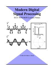
Frequency Responseof FIR FiltersChapter6This chapter continues the study of FIR filters from Chapter 5,but the emphasis is frequency response, which relates to how thefilter responds to an input of the formxn =e jˆ 0n – n .A fundamental result we shall soon see, is that the frequencyresponse and impulse response are related through an operationknown as the Fourier transform. The Fourier transform itself isnot however formally studied in this chapter.Sinusoidal Response of FIR Systems• Consider an FIR filter when the input is a complex sinusoidof the formxn = Ae j e jˆ 0n – n , (6.1)where it could be that xn was obtained by sampling thecomplex sinusoid xt Ae j e j 0t= and ˆ 0 = 0T s• From the difference equation for an M + 1tap FIR filter,Myn b kxn – kb kAe j e jˆ 0 n – k= =k = 0Mk = 0(6.2)ECE 2610 Signal and Systems 6–1

Sinusoidal Response of FIR Systemsyn =Ae j e jˆ 0nk = 0b ke j– ˆ 0kAe j e jˆ 0n jˆ= He 0– n where we have defined for arbitrary ˆM(6.3)He jˆM = b ke jk = 0– ˆ k(6.4)to be the frequency response of the FIR filter• Note: The notation He jˆ is used rather than say Hˆ, tobe consistent with the z-transform which will defined inChapter 7, and to emphasize the fact that the frequencyresponse is periodic, with period 2 (more on this later)– Note: e jˆ = cosˆ+jsinˆ, where sine and cosine areboth mod2functions• Returning to (6.2), the implication is that when the input is acomplex exponential at frequency ˆ 0 , the output is also acomplex exponential at frequency ˆ 0• The complex amplitude (magnitude and phase) of the input ischanged as a result of passing through the system– The frequency response at ˆ 0 multiplies the input amplitudeto produce the output– It is not true in general that yn = He jˆ 0xn , butonly for the special case of xn a complex sinusoidapplied starting at –ECE 2610 Signals and Systems 6–2

Sinusoidal Response of FIR Systems• The frequency response is a complex function of ˆgenerally viewed in either polar or rectangular formthat isHe jˆ He jˆ e j H ejˆ=(6.5)= ReHe jˆ+jImHe jˆ– The polar or magnitude and phase form is perhaps themost common• The polar form offers the following interpretation ofterms of xn , when the input is a complex sinusoidyn == e j H ejˆHe jˆ Ae j H ejˆHe jˆyn in(6.6)– Here we see that the input amplitude is multiplied by thefrequency response amplitude, and the input phase hasadded to it the frequency response phase– The output amplitude expression means that isalso termed the gain of an LTI systemAe j e jˆ n + jˆ n eHe jˆExample: = 11311 b k• The frequency response of this FIR filter is– b ke jˆ k=He jˆ=4k = 0–1 + e jˆ+ 3e – j2ˆ+ e – j3ˆ+e – j4ˆECE 2610 Signals and Systems 6–3

Sinusoidal Response of FIR Systems– We have used the inverse Euler formula for cosine twice• For this particular filter we have thatWhy?– = e j2ˆHe jˆ=He jˆ–e j2ˆe j2ˆe jˆ –+ + 3 + e jˆ+–e j2ˆ2cos2ˆ + 2cosˆ + 3 = 3 + 2cosˆ + 2cos2ˆHe jˆ=– 2ˆ• Use MATLAB to plot the magnitude and phase response>> w = 0:2*pi/200:2*pi;>> H = exp(-j*2*w).*(3 + 2*cos(w) + 2*cos(2*w));>> subplot(211)>> plot(w,abs(H))>> axis([0 2*pi 0 8])>> grid>> ylabel('Magnitude')>> subplot(212)>> plot(w,angle(H))>> axis([0 2*pi -pi pi])>> grid>> ylabel('Phase (rad)')ECE 2610 Signals and Systems 6–4

Sinusoidal Response of FIR Systems>> xlabel('hat(\omega) (rad)')8Magnitude6423.248Phase (rad)00 1 2 3 4 5 620−2–-20 1 2 3 4 5 6hat(ω) (rad)22Example: Findyn for Input• The input frequency isthe phase is = 0xn = 5e j1 nˆ 0 = 1rad, the amplitude is 5, and• Assuming xn is input to the 4-tap FIR filter in the previousexample, the filter output isyn = 3 + 2cos1+ 2cos2 1e j1 2= 16.2415e – j2 e jn• The amplitude response or gain at ˆ 0 = 1 is He j1 =3.248; why?– 5e j1 nECE 2610 Signals and Systems 6–5

• We now use (6.10) to simplify (6.9)yn =A-- He jˆ 0 j ˆ e 0n + 2 ASuperposition and the Frequency Response-- H* e jˆ 0 j+ e2– ˆ 0n + = AH e jˆ 0e j ˆ 0n + + He jˆe – j ˆ 0n + +He jˆ+ ------------------------------------------------------------------------------------------------2(6.11)yn AH e jˆ 0 cosˆ 0n + + He jˆ 0=ˆ• We see that when a real sinusoid passes through an LTI system,such as an FIR filter (having real coefficients), the outputis also a real sinusoid which has picked up the magnitudeand phase of the system at = ˆ 0• The generalization (sum of sinusoids) of this result is whenNxn = X 0+ X kcosˆ kn + X k, (6.12)k = 1then the corresponding LTI system output isyn =X 0He j0 +Nk = 1X kHe jˆ k cos ˆ kn+ X k+He jˆ k(6.13)ECE 2610 Signals and Systems 6–7

Superposition and the Frequency ResponseExample: Three Inputs with• The input is• The frequency response is• The input frequencies areHe j0He j 4He j 3• Thusb k= 1– 11xn 10 4 --n+--= + cos + 3 --n –--48cos 3 4– 1 – e jˆ –= + e j2ˆHe jˆ–e jˆ– 1 + 2cosˆ>> w = 0:pi/200:pi;>> H = 1 - exp(-j*w) + exp(-j*2*w);>> subplot(211)>> plot(w,abs(H))>> grid>> hold>> plot([pi/4 pi/4],[0 3],'r')=ˆ k = 0 43 = e – j0 – 1 + 2cos0 = 1 = e – j 4 – 1 + 2cos 4 = 0.4142e – j 4 = e – j 3 – 1 + 2cos 3 = 0yn = 10 1 + 4 0.4142 cos --n +-- –-- 4 8 4= 10 + 1.6569 cos --n –-- 4 8ECE 2610 Signals and Systems 6–8

Superposition and the Frequency Response>> plot([pi/3 pi/3],[0 3],'r')>> ylabel('Magnitude')>> subplot(212)>> plot(w,angle(H))>> grid>> hold>> plot([pi/4 pi/4],[-2 3],'r')>> ylabel('Phase (rad)')>> xlabel('Digital Frequency \omega')He jˆ 32.5Magnitude21.510.4142 00.500 0.5 1 1.5 2 2.5 3 3.532--4--3Phase (rad)10−1–--4−20 0.5 1 1.5 2 2.5 3 3.5Digital Frequency ω• We have used frequency domain analysis to complete thisexample• We could also perform a time domain analysis using sayMATLAB’s filter function (more on this in the next section)ECE 2610 Signals and Systems 6–9

Steady-State and Transient ResponseSteady-State and Transient Response• The frequency response definition relies on the fact that thesupport interval for the complex sinusoid input is – • In a computer simulation or in a real-time signal processingapplication, it is not practical to consider input signals whichbegin at –• Consider an input that begins at n = 0 using the unit stepfunction to turn on the inputwhereX=Ae jxn un and= Xe jˆ n un 1, n 00, otherwise(6.14)(6.15)• For an LTI FIR system, the convolution sum formula yieldsMyn b kXe jˆ n – k= un – k k = 0hk (6.16). . .0 Mun – kn 0kkECE 2610 Signals and Systems 6–10

• The sum of (6.16) is composed of three cases• Whenyn =n 00, n 0n–b ke jˆ k jˆ Xe n ,0 n Mk = 0 M–b ke jˆ k jˆ n Xe , n Mk = 0Steady-State and Transient Responsethe input is not present, so the output is zero(6.17)• When 0 n M the input has partially engaged the filter andthe output produced is the transient response• When n M, the output is in steady-state, since the input hasfully engaged the filter– Note that the steady-state response is also equivalent tosayingyn He jˆXe jˆ(6.18)– Note also that the steady-state output assumes that theinput is always Xe jˆ nfor n 0Example: Revisit Three Inputs with= n Mb k= 1– 11• The frequency domain analysis used in the previous exampleobtained just the steady-state portion of the output• We can evaluate the convolution sum or use MATLAB’s filterfunction to obtain a solution of the form described in (6.17)ECE 2610 Signals and Systems 6–11

Steady-State and Transient Response>> n = -5:20;>> x = (10 + 4*cos(pi/4*n+pi/8) + ...3*cos(pi/3*n-pi/4)).*ustep(n,0);>> y = filter([1 -1 1],1,x);>> subplot(211)>> stem(n,x,'filled')>> grid>> ylabel('x[n]')>> subplot(212)>> stem(n,y,'filled')>> holdCurrent plot released>> stem(n,y,'filled')>> grid>> ylabel('y[n]')>> xlabel('Sample Index n')2015x[n]1050−5 0 5 10 15 202015TransientIntervaly[n]1050Steady-state−5−5 0 5 10 15 20Sample Index nECE 2610 Signals and Systems 6–12

• The function ustep() is defined as:Steady-State and Transient Responsefunction x = ustep(n,n0)% function x = ustep(n,n0)%% Generate a time shifted unit step sequencex = zeros(size(n));i_n0 = find(n >= n0);x(i_n0) = ones(size(i_n0));• If we consider just the steady-state portion of the output weshould be able to discern the same output as obtained fromthe frequency domain analysis of the previous example1211.52 1.6568 = 3.31381110.5y[n]109.5DC = 10y[n] peaklag 1/2sample =/898.585 10 15 20x[n] cos() peakSample Index n• The measurements above agree with the earlier exampleECE 2610 Signals and Systems 6–13

Properties of the Frequency ResponseProperties of the Frequency ResponseRelation to Impulse Response and Difference Equation• In the definition of the frequency response, He jˆ , for anFIR filter, the coefficients were utilized• Similarly given the frequency response, the impulse responsecan be foundhn • In Chapter 5 we saw that the impulse response and differenceequation are directly related, so in summary given one theother two are easy to obtainExample:• Given sayMwe immediately see that• The difference equation is• The frequency response isb kTime Domain Frequency Domain= hk n– kHe jˆ– hk e jˆ k =hn k = 0hn yn He jˆ==He jˆMk = 02n + 3n – 1 – 2n – 2 = 23 – 2b k2xn + 3xn–1 – 2xn–2– ˆ = 2+3e j–2e – j2ˆECE 2610 Signals and Systems 6–14

Properties of the Frequency ResponseExample: Difference Equation from• Suppose that• We immediately can write thatand• It could have been thatstarted in this formExample:hn yn He jˆHe jˆ• We need to convert the sine form back to complex exponentials• The impulse response is thus?– 2ˆHe jˆ = 1+ 4e j +=He jˆ=4e – j4ˆn + 4n – 2 + 4n – 4xn + 4xn–2 + 4xn–4 1 8e j2ˆ ----------------------------+ = + 2 –= 1+8e j2ˆcos2ˆ– e j2ˆ– 2j ˆ 2e jˆ 2= sin 2je j ˆ 2=He jˆ=– e jˆ 2–1 – e jˆ–e j2ˆe – jˆ 2– --------------------------------- 2j ECE 2610 Signals and Systems 6–15

Properties of the Frequency Response• The difference equation is?Periodicity ofHe jˆ • For any discrete-time LTI system, the frequency response isperiodic, that isHe j ˆ + 2 He jˆ• The proof for FIR filters followsHe j ˆM + 2– b ke j ˆ + 2=k = 0=Mk = 0–b ke jˆ (6.19)(6.20)• This result is consistent with the fact that sinusoidal signalsare insensitive to 2 frequency shifts, i.e.,• In summary, the frequency response is unique on at most a2 interval, say in particular the interval – ˆ Conjugate Symmetry• The frequency response He jˆ is in general a complexquantity, in most cases obeys certain symmetry propertiese – j21=He jˆxn Xe j ˆ + 2nXe jˆ n j2n= = e =Xe jˆ nECE 2610 Signals and Systems 6–16

Properties of the Frequency Response• In particular if the coefficients of a digital filter are real, that*is b k= b kor hk = h * k, thenproof–Conjugate Symmetry: He jˆ = H * e jˆH * e jˆ – b ke jˆ k * M* jˆ k= = b k e =• A consequence of conjugate symmetry is that(6.21)(6.22)(6.23)– We say that the magnitude response is an even function ofˆ and the phase is an odd function of ˆ• It also follows thatMk = 0Mk = 0b ke j– –ˆ kk = 0–He jˆ• When plotting the frequency response we can use the abovesymmetry to just plot over the interval 0 ˆ =He – jˆ = He jˆHe – jˆ = – He j ˆReHe – jˆ = ReHe jˆ(6.24)ImHe – jˆ = – ImHe jˆ– We say that the real part response is an even function of ˆand the imaginary part is an odd function of ˆECE 2610 Signals and Systems 6–17

Graphical Representation of the Frequency ResponseGraphical Representation of the FrequencyResponse• A useful MATLAB function for plotting the frequencyresponse of any discrete-time (digital) filter is freqz()• The interface to freqz() is similar to filter() in that aand b vectors are again required– Recall that the b vector holds the FIR coefficientsand for FIR filters we set a = 1.>> help freqzFREQZ Digital filter frequency response.[H,W] = FREQZ(B,A,N) returns the N-point complex frequency responsevector H and the N-point frequency vector W in radians/sample ofthe filter:jw -jw -jmwjw B(e) b(1) + b(2)e + .... + b(m+1)eH(e) = ---- = ------------------------------------jw -jw -jnwA(e) a(1) + a(2)e + .... + a(n+1)egiven numerator and denominator coefficients in vectors B and A. Thefrequency response is evaluated at N points equally spaced around theupper half of the unit circle. If N isn't specified, it defaults to512.[H,W] = FREQZ(B,A,N,'whole') uses N points around the whole unit circle.H = FREQZ(B,A,W) returns the frequency response at frequenciesdesignated in vector W, in radians/sample (normally between 0 and pi).[H,F] = FREQZ(B,A,N,Fs) and [H,F] = FREQZ(B,A,N,'whole',Fs) returnfrequency vector F (in Hz), where Fs is the sampling frequency (in Hz).H = FREQZ(B,A,F,Fs) returns the complex frequency response at thefrequencies designated in vector F (in Hz), where Fs is the samplingfrequency (in Hz).FREQZ(B,A,...) with no output arguments plots the magnitude andunwrapped phase of the filter in the current figure window.See also filter, fft, invfreqz, fvtool, and freqs.b kECE 2610 Signals and Systems 6–18

Graphical Representation of the Frequency ResponseExample: Delay System yn = xn – n 0• This filter contains one coefficient, b n0= 1, soHe jˆ e jˆ n=0=>> [H,w] = freqz([0 0 0 0 1],1);>> subplot(211)>> plot(w,abs(H))>> axis([0 pi 0 1.2]); grid>> ylabel('Magniude Response')>> subplot(212)>> plot(w,angle(H))>> axis([0 pi -pi pi]); grid>> ylabel('Phase Response (rad)')>> xlabel('hat(\omega)')–1–ˆ n 0Magnitude Response10.5Constant magnitude (gain) responsen 0 = 400 0.5 1 1.5 2 2.5 3Phase Response (rad)2Linear Phase0–4ˆMATLABwraps the−2phase mod2–0 0.5 1 1.5 2 2.5 3hat(ω)ECE 2610 Signals and Systems 6–19

Graphical Representation of the Frequency ResponseExample: First-Difference System• The frequency response isHe jˆyn xn –xn – 1– = 1 – e jˆ= 1 – cosˆ+jsinˆ>> w = -pi:pi/100:pi;>> H = freqz([1 -1],1,w); %use a custom w axis>> subplot(211)>> plot(w,abs(H))>> axis([-pi pi 0 2]); grid; ylabel('Magniude Response')>> subplot(212)>> plot(w,angle(H))>> axis([-pi pi -2 2]); grid;>> ylabel('Phase Response (rad)')>> xlabel('hat(\omega)')2Magnitude Response1.510.52 sinˆ 20−3 −2 −1 0 1 2 3=Phase Response (rad)210−1atan sinˆ--------------------- 1 – cosˆ−2−3 −2 −1 0 1 2 3hat(ω)ECE 2610 Signals and Systems 6–20

Graphical Representation of the Frequency ResponseExample: A Simple Lowpass Filteryn = xn + 2xn–1 + xn – 2• The frequency response isHe jˆ– = 1 2e jˆe j2ˆ=>> w = -pi:pi/100:pi;>> H = freqz([1 2 1],1,w);>> subplot(211)>> plot(w,abs(H))>> axis([-pi pi 0 4]); grid;>> ylabel('Magnitude Response')>> subplot(212)>> plot(w,angle(H))>> axis([-pi pi -pi pi]); grid;>> ylabel('Phase Response (rad)')>> xlabel('hat(\omega)')–+ + e jˆ2+2cosˆMagnitude Response43212 + 2cosˆ0−3 −2 −1 0 1 2 3Phase Response (rad)2–ˆ0−2−3 −2 −1 0 1 2 3hat(ω)ECE 2610 Signals and Systems 6–21

Cascaded LTI SystemsCascaded LTI Systems• Cascaded LTI system were discussed in Chapter 5 from thetime-domain standpoint• In the frequency-domain there is an alternative view of theinput/output relationships• To begin with consider againxn e jˆ n – n • With LTI #1 followed by LTI #2, the output at frequencyy 1n===H 2e jˆH 2e jˆH 1e jˆH 1e jˆe jˆ ne jˆ n(6.25)ˆis(6.26)ECE 2610 Signals and Systems 6–22

Cascaded LTI Systems• With LTI #2 followed by LTI #1, the output at frequencyy 2n==H 1e jˆH 1e jˆH 2e jˆH 2e jˆe jˆ ne jˆ nis(6.27)• Since H 1e jˆH 2e jˆ = H 2e jˆH 1e jˆ, it follows thaty 1n= y 2n, and we have established that the frequencyresponse for a cascaded system is simply the product of thefrequency responsesˆH cascadee jˆ = He jˆ = H 1e jˆH 2e jˆ(6.28)• We have also shown that a convolution in the time-domain isequivalent to a multiplication in the frequency-domainhn Example: Two System Cascade• ConsiderTime Domain Frequency Domain= h 1n*h 2n H 1e jˆH 2e jˆ = He jˆH 1e jˆ = 1 + e jˆH 2e jˆ–= 1+ 2e jˆ+• The cascade frequency response isHe jˆ–e j2ˆ 1 + e jˆ–= 1+ 2e jˆ+–1 3e jˆ –= + + 3e j2ˆ+–e j2ˆ–e j3ˆ(6.29)ECE 2610 Signals and Systems 6–23

Moving Average Filtering• Given the cascade frequency response we can easily convertback to the impulse response of the cascade difference equationhn = n + 3n – 1+ 3n – 2 + n – 3andyn = xn + 3xn–1 + 3xn–2 + xn – 3• Check h 1n*h 2nMoving Average Filtering• The moving average filter occurs frequency enough that weshould consider finding a general expression for the frequencyresponse• The difference equation for an L-point averager isyn • The frequency response is=L – 11-- xn – kL k = 0(6.30)He jˆ=L – 11 –-- e jˆ kL k = 0(6.31)ECE 2610 Signals and Systems 6–24

• This sum is known as a finite geometric series• It can be shown (discussed in class) thatMoving Average FilteringL – 1 kk = 01 – L-------------- 1 – , 1L, = 1 (why?)• Apply (6.32) to (6.31) by setting==–e jˆ(6.32)He jˆ===1-- 1 e – jˆ L– ---------------------L–1 – e jˆ --1 e – jˆ L 2e jˆ L 2e – jˆL 2 – ---------------------------------------------------------------L–e jˆ 2e jˆ 2e – jˆ 2 – --------------------------sinˆ L 2 – jˆ L – 1 eLsinˆ 2 2(6.33)• Notice that the phase response is composed of a linear term–e jˆ L – 1 2and due to the sign changes of sinˆ L 2/Lsinˆ 2• In MATLABD Le jˆ = diricˆ L=--------------------------sinˆ L 2Lsinˆ 2can be used for analyzing moving average filtersECE 2610 Signals and Systems 6–25

Moving Average FilteringPlotting the Frequency Response• The frequency response can be plotted most easily usingMATLAB’s freqz() function• Consider a 10-point moving average>> w = -pi:pi/500:pi;>> H = freqz(ones(1,10)/10,1,w);>> subplot(211)>> plot(w,abs(H))>> grid; axis([-pi pi 0 1])>> ylabel('Magnitude Response')>> subplot(212)>> plot(w,angle(H))>> grid; axis([-pi pi -pi pi])>> ylabel('Phase Response (rad)')>> xlabel('hat(\omega)')Magnitude Response10.5L = 100−3 −2 −1 0 1 2 3 2 4 3--5-----5ˆ=-----52-----L-----5Phase Response (rad)20−2–e j4.5 ˆon this segment−3 −2 −1 0 1 2 3hat(ω)ECE 2610 Signals and Systems 6–26

Filtering Sampled Continuous-Time SignalsFiltering Sampled Continuous-Time Signals• Consider the system model as shown below• Suppose thatxt = – t Xe jt• We know that after sampling we have(6.34)xn xnT s Xe jnT s= = =Xe jˆ n(6.35)• The key relationship to connect the continuous-time and thediscrete-time quantities isˆ = T s= 2 --ffˆ= ---- = ˆ f sT s= -----------ˆ=2T s(6.36)• As long as the input analog frequency satisfies the samplingtheorem, i.e., T sor f f s 2, the output of the discrete-timesystem will bef s-----ˆ f2 sECE 2610 Signals and Systems 6–27

Filtering Sampled Continuous-Time Signalsyn =He jˆXe jˆ n(6.37)• We can write yn in terms of the analog frequency variable via ˆ = T syn =He jT s Xe jT sn(6.38)• At the output of the D-to-C converter we have the reconstructedoutputyt ==He jT s Xe jtHe j2f f sXe j 2f f st(6.39)where f is the input analog sinusoid frequency (perhaps a betternotation would be f 0 0ˆ 0 )Example: Lowpass Averager• Consider a 5-point moving average filter wrapped upbetween a C-to-D and D-to-C system• We assume a sampling rate of 1000 Hz and an input composedof two sinusoidsxt =cos2100t+3cos2300t• Find the system frequency response in terms of the analogfrequency variable f, and find the steady-state output yt • We will use freqz() to obtain the frequency response>> w = -pi:pi/100:pi;>> H = freqz(ones(1,5)/5,1,w);>> subplot(211)ECE 2610 Signals and Systems 6–28

Filtering Sampled Continuous-Time Signals>> plot(w,abs(H))>> axis([-pi pi 0 1]); grid>> ylabel('Magnitude Response')>> subplot(212)>> plot(w,angle(H))>> axis([-pi pi -pi pi]); grid>> ylabel('Phase Response (rad)')>> xlabel('hat(\omega)')Magnitude Response10.5Magnitude and Phase Plots of He jˆ 0−3 −2 −1 0 1 2 3Phase Response (rad)20−2−3 −2 −1 0 1 2 3hat(ω)>> subplot(211)>> plot(w*1000/(2*pi),abs(H))>> grid>> ylabel('Magnitude Response')>> subplot(212)>> plot(w*1000/(2*pi),angle(H))>> grid>> ylabel('Phase Response (rad)')>> xlabel('f (Hz)')ECE 2610 Signals and Systems 6–29

Filtering Sampled Continuous-Time SignalsMagnitude Response10.5Magnitude and Phase Plots of He j2f f s 0−500 −400 −300 −200 −100 0 100 200 300 400 500Phase Response (rad)420−2−4−500 −400 −300 −200 −100 0 100 200 300 400 500f (Hz)• The output yt will be of the same form as the input xt ,except the sinusoids at 100 and 300 Hz need to have the filterfrequency response applied– Note 100 Hz and 300 Hz < 1000/2 = 500 Hz (no aliasing)• To properly apply the filter frequency response we need toconvert the analog frequencies to the corresponding discretetimefrequencies100Hz 2 -----------1001000= 2 0.1 = 0.2300Hz 2 -----------3001000= 2 0.3 = 0.6(6.40)ECE 2610 Signals and Systems 6–30

• The frequency response foraverage filter isFiltering Sampled Continuous-Time Signalsin the general moving• The frequency response at these two frequencies isHe j0.2 He j0.6 (6.41)sin2.50.2= --------------------------------------e – j20.2 = 0.6472e – j0.45sin0.2 2(6.42)sin2.50.6= --------------------------------------e – j20.6 = – 0.2472e – j1.25sin0.6 2>> diric(0.2*pi,5)ans = 0.6472He jˆ>> diric(0.6*pi,5)=L = 5sin2.5ˆ5 --------------------------e – j2ˆsinˆ 2 0.2472e – j0.2ans = -0.2472 % also = 0.2472 at angle +/- pi• The filter output yn isyn = 0.6472cos0.2n – 0.4+ 0.7416cos0.2n – 1.2 + and the D-to-C output isyt =0.6472cos2100t – 0.4+ 0.7416cos2300t – 0.2(6.43)(6.44)ECE 2610 Signals and Systems 6–31

Filtering Sampled Continuous-Time SignalsInterpretation of Delay• In the study of the moving average filter, it was noted thatwhereD Le jˆHe jˆ• The pure delay systemhas impulse responseand has frequency response D Le jˆ –e jˆ L – 1=is a purely real functionyn = xn – n 0hn = n–n 0– e jn 0ˆ=He jˆ• We also know that the impulse response of two systems incascade ishn He jˆh 1n*h 2n• The L-point moving average filter thus incorporates a delayof L – 1 2 samples• Viewed as a cascade of subsystemsHe jˆ– If L is odd then the delay is an integer= = H 1e jˆ 2H 2e jˆ D Le jˆ – e jˆ L – 1= – If L is even then the delay is an odd half integer(6.45)ECE 2610 Signals and Systems 6–32 2