Frequency Response of FIR Filters

More documents

Recommendations

Info

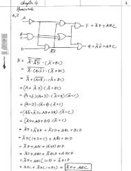
Graphical Representation of the Frequency ResponseGraphical Representation of the FrequencyResponse• A useful MATLAB function for plotting the frequencyresponse of any discrete-time (digital) filter is freqz()• The interface to freqz() is similar to filter() in that aand b vectors are again required– Recall that the b vector holds the FIR coefficientsand for FIR filters we set a = 1.>> help freqzFREQZ Digital filter frequency response.[H,W] = FREQZ(B,A,N) returns the N-point complex frequency responsevector H and the N-point frequency vector W in radians/sample ofthe filter:jw -jw -jmwjw B(e) b(1) + b(2)e + .... + b(m+1)eH(e) = ---- = ------------------------------------jw -jw -jnwA(e) a(1) + a(2)e + .... + a(n+1)egiven numerator and denominator coefficients in vectors B and A. Thefrequency response is evaluated at N points equally spaced around theupper half of the unit circle. If N isn't specified, it defaults to512.[H,W] = FREQZ(B,A,N,'whole') uses N points around the whole unit circle.H = FREQZ(B,A,W) returns the frequency response at frequenciesdesignated in vector W, in radians/sample (normally between 0 and pi).[H,F] = FREQZ(B,A,N,Fs) and [H,F] = FREQZ(B,A,N,'whole',Fs) returnfrequency vector F (in Hz), where Fs is the sampling frequency (in Hz).H = FREQZ(B,A,F,Fs) returns the complex frequency response at thefrequencies designated in vector F (in Hz), where Fs is the samplingfrequency (in Hz).FREQZ(B,A,...) with no output arguments plots the magnitude andunwrapped phase of the filter in the current figure window.See also filter, fft, invfreqz, fvtool, and freqs.b kECE 2610 Signals and Systems 6–18
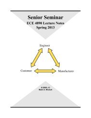
Graphical Representation of the Frequency ResponseExample: Delay System yn = xn – n 0• This filter contains one coefficient, b n0= 1, soHe jˆ e jˆ n=0=>> [H,w] = freqz([0 0 0 0 1],1);>> subplot(211)>> plot(w,abs(H))>> axis([0 pi 0 1.2]); grid>> ylabel('Magniude Response')>> subplot(212)>> plot(w,angle(H))>> axis([0 pi -pi pi]); grid>> ylabel('Phase Response (rad)')>> xlabel('hat(\omega)')–1–ˆ n 0Magnitude Response10.5Constant magnitude (gain) responsen 0 = 400 0.5 1 1.5 2 2.5 3Phase Response (rad)2Linear Phase0–4ˆMATLABwraps the−2phase mod2–0 0.5 1 1.5 2 2.5 3hat(ω)ECE 2610 Signals and Systems 6–19
Page 1 and 2: Frequency Responseof FIR FiltersCha
Page 3 and 4: Sinusoidal Response of FIR Systems
Page 5: Sinusoidal Response of FIR Systems>
Page 8 and 9: Superposition and the Frequency Res
Page 10 and 11: Steady-State and Transient Response
Page 12 and 13: Steady-State and Transient Response
Page 14 and 15: Properties of the Frequency Respons
Page 16 and 17: Properties of the Frequency Respons
Page 20 and 21: Graphical Representation of the Fre
Page 22 and 23: Cascaded LTI SystemsCascaded LTI Sy
Page 24 and 25: Moving Average Filtering• Given t
Page 26 and 27: Moving Average FilteringPlotting th
Page 28 and 29: Filtering Sampled Continuous-Time S
Page 30 and 31: Filtering Sampled Continuous-Time S
Page 32: Filtering Sampled Continuous-Time S

Frequency Response of FIR Filters

You also want an ePaper? Increase the reach of your titles

Delete template?

Save as template?