Design and Simulation of Active Suspension System by Using Matlab

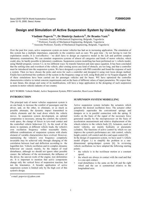
Seoul 2000 FISITA World Automotive CongressJune 12-15, 2000, Seoul, KoreaF2000G269Design and Simulation of Active Suspension System by Using MatlabVladimir Popovic 1) *, Dr Dimitrije Jankovic 2) , Dr Branko Vasic 3)1) Assistant, Faculty of Mechanical Engineering, Belgrade, Yugoslavia2) Professor, Faculty of Mechanical Engineering, Belgrade, Yugoslavia3) Associate Professor, Faculty of Mechanical Engineering, Belgrade, YugoslaviaOver the past few years, active suspension system on motor vehicles has had an in increasing application. The simulation ofthis system has a multiple importance, especially in the countries such as ours: We gain time - by not having to wait forexploitation results; It is cost-effective - we don't have to design an expensive model in the Lab and perform complexlaboratory examinations; We can simulate suspension systems of almost all categories and kinds of motor vehicles, whichcould, also, be hardly possible in laboratory conditions. Suspension system modelling has been performed on ¼ vehicle model,using Matlab program, version 5.2, in two different ways: by transfer function and state-space equation. It has been concludedthat the settling time and overshoot of the vehicle, after coming across any kind of obstacle, are too long, and that a controllermust be introduced into the suspension system. We have designed a system with PID controller and found the response of sucha system. Then we have chosen the poles and zeros for such a controller and designed it using root locus design method.Finally have performed the synthesis of the system in the frequency range as well, using Bode plot or via Nyquist diagram. Allof these simulations have been carried out for passenger vehicles and for buses. WE have optimized the controllercharacteristics relative to initial concrete requirements and on the basis of different values of input parametres. We expect that,in near future, this design and some of its modifications, will have a large application in the designing of such suspensionsystems in motor vehicles industry of our country.KEY WORDS: Vehicle Model, Active Suspension System, PID Controller, Root Locus MethodINTRODUCTIONThe principal task of motor vehicles suspension system ison one hand, to increase the comfort of passengers and thedriver, and, on the other, to eliminate, or as much aspossible attenuate, the dynamic impact transmitted tovehicle elements and the road down which the vehiclemoves. In suspension system development, an optimalcompromise is necessary, among the comfort, the system'swork space, the change of forces in tyre-road contact andthe controlled vehicle behaviour [1]. As the result of thedesire to maintain, at different vehicle loads, the vehicle'sown oscillation frequency within reasonable limits,different combinations of suspension systems with elasticelement of variable characteristics have evolved. However,maintaining the vehicle's own frequency completelyinvariable may be achieved only through changing of thecorrelation between load and deflection according to thelogarithm law. Vehicle oscillation and its complex dynamicbehaviour are caused, mainly, by the impact of roaddisturbance, although we should not ignore other possiblecauses: the influence of the environment, the influence ofthe driver, the uneven work of the engine, tyre deformitiesetc. It is important to mention that active componentschange only the vertical force of suspension reaction, butnot the kinematics. A broader application of activesuspension system is limited only by the high cost of thissystem's design.SUSPENSION SYSTEM MODELLINGActive suspension system includes the actuators whichgenerate the desired oscillation force. The actuator eithercompletely supersedes the conventional springs anddampers or is in parallel connection with the spring. Itworks on the basis of the signal of the necessary forcegenerated usually by the microprocessor on the basis ofacceleration measurement and relative displacement of thewheels relative to the vehicle body [2]. Actuators, used onmotor vehicles, are mainly hydraulic or pneumaticcylinders. The functions of active control by which we canimprove the system's performance are: ride control, vehicleheight control, roll control and dive and squat control [8].In the design of suspension system, we have used ¼ vehiclemodel (Figure 1.) to simplify the problem to a onedimensionalspring-damper system [6]. In reviewingvehicle oscillations we have adopted the following startingpoints:∗ the vehicle is in the rectilinear motion at a constantspeed;∗ the wheels are always in contact with the road and thatis a one-spot contact;∗ road disturbance is the same on the left and the rightwheel and the car is symmetrical relative to thelongitudinal axis;* e-mail: popovicv@yahoo.com1

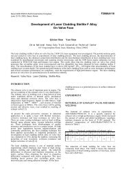
∗ mass distribution coefficient is approximately 1.Although the real characteristics of the suspension system(k1, b1) are non-linear, we have adopted constant values forthem in this paper which, without any significant error,enable the linearization of the model. The same has beendone for k2 and b2. The designations on Figure 1. have thefollowing meanings:∗ body mass (m1) = 2250 (285) kg;∗ suspension mass (m2) = 290 (60) kg;∗ spring constant of suspension system (k1) = 72000(25400) N/m;∗ spring constant of wheel and tyre (k2) = 450000(200000) N/m;∗ damping constant of suspension system (b1) = 315(1300) Ns/m;∗ damping constant of wheel and tyre (b2) = 13500 (700)Ns/m;∗control force (F a ) = force from the controller we aregoing to design.The data that we used during the simulation are for a busand a passenger car (in the brackets). We have performedsimulations for both categories of vehicles (M 3 and M 1 -according to ECE Regulations), but have presented hereonly the results obtained for the bus. However, the adoptedconclusions also apply to the passenger car.BodyMassSuspensionMassk 1Figure 1. - ¼ Vehicle ModelWhen the vehicle is experiencing any road disturbance, thebody should not have large oscillations, and the oscillationsshould dissipate quickly. This, at the same time, is ourprincipal task. Since the distance x 1 -W is very difficult tomeasure, and the deformation of the tyre x 2 -W is negligible,we will use the distance x 1 -x 2 instead of x 1 -W as the outputin our problem. The road disturbance W will be simulatedby a step input. This step could represent the vehiclecoming out of a pothole. We want to design a feedbackcontroller so that the output x 1 -x 2 has an overshoot less than5% and a settling time shorter than 5 seconds. For example,when the vehicle runs onto a 10 cm high step, the body willoscillate within a range of ±5 mm and return to a smoothride within 5 seconds.MODELLING BY USING TRANSFER FUNCTIONk 2The assessment of the quality of automatic regulationsystem behaviour essentially boils down to estimating theerror between a predetermined value and the real value ofthe controlled variable. The knowing of this error at anypoint would give a complete information on the features ofthe observed system. Due to the diversity of the laws of theF ab 2b 1X 1X 2Wsystem's input change, which might occur in the normalwork regime, such an approach, based on estimation of thecurrent values of error, is inappropriate speaking from theaspect of practice. Therefore, it is preferable to make anestimation of the relevant system characteristics on thebasis of the features it manifests at its being disturbed bythe typical input signals. With such an approach, the systemis being defined both in the stationary and transitional workregime. On the basis of Figure 1. and the Newton's Law, wecan obtain the following dynamic equations, whichrepresent the mathematical model of the dynamic system:m 1 x1 = −b1(x1 − x2)− k1(x1− x2)+ Fa(1)m2x2= b1(x1 − x2)+ k1(x1− x2)+ b2(W− x2)+(2)+ k 2(W− x2)− FaThe solving of these equations is, to a large extent,simplified by the application of Laplace transforms. Withthe help of these, we can immediately obtain the solutionfor the linear differential equations with constantcoefficients for the given initial conditions. The transformsprovide the representation of the system in the form of anappropriate block diagram. Although Laplace transformsmay not be the most ideal solution due to the possibility ofcomplex algebra occurrence, the majority of procedures forthe synthesis and analysis of the automatic control system,more or less, relies on the application of LaplaceTransforms. This approach is not possible with linear nonstationarysystems, in which one or several parametreschange in time [4]. Let's assume that all the initialconditions are zeroes, so these equations represent thesituation when a wheel goes up a bump. The dynamicequations above can be expressed in a form of transferfunctions by taking Laplace Transform of the aboveequations. The derivation from above equations of theTransfer functions G 1 (s) and G 2 (s) of output, x 1 -x 2 , and twoinputs, F a and W, are as follows:M⎡ 2(m ⎤1s+ b1s+ k1)− (b1s+ k1)⎢⎥ *2⎢⎣− (b1s+ k1)m2s+ (b1+ b2)s+(k1+ k 2)⎥⎦(3)⎡X1(s)⎤ ⎡ Fa(s) ⎤* ⎢ ⎥ = ⎢⎥⎣X2(s)⎦ ⎣(b2s+k 2)W(s)− Fa(s) ⎦2∆ = det[ M]= (m1s+ b1s+ k1) *(4)22* (m2s+ (b1+ b2)s+(k1+ k 2))− (b1s+ k1)Then, we find the inverse of the matrix A and multiply withinputs F a (s) and W(s) on the right hand side as thefollowing:⎡m2s2+ 2⎤⎢b 1 b 2 s + (b 1 k 2 + b 2 k 1 )s+k 1 k 2 ⎥⎡X1(s)⎤ 1 ⎢+b 2 s+k 2⎥⎢ ⎥ = **X2(s)⎢m3(m b2 ⎥⎣ ⎦ ∆⎢ 2 1 b 2 s + 1 k 2 + 1 b 2 )s +− m 1 s⎥⎢(b1k2 b2k1)s⎥⎣+ + + k1k2 ⎦⎡F a (s) ⎤* ⎢ ⎥(5)⎣W(s)⎦When we want to consider input F a (s) only, we set W(s)=0.Thus we get the transfer function G 1 (s) as the following:2X1(s)− X 2(s)(m1+ m2)s+ b2s+k 2G 1(s)==(6)Fa(s)∆2

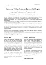
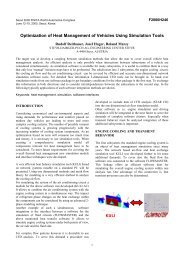
When we want to consider input W(s) only, we set F a (s)=0.Thus we get the transfer function G 2 (s) as the following:3 2X1(s)− X 2(s)− m1b2s− m1k2sG 2(s)==(7)W(s)∆We can put the above Transfer Function equations (6) and(7) into Matlab by defining the numerator and denominatorof Transfer Functions in the form, nump/denp for actuatedforce input and nums/dens for disturbance input, of thestandard transfer function G 1 (s) and G 2 (s):numpnumsG1 (s) = G2(s)=(8)denpdensOn the basis of above equations we have created an m-filewith the data that we have found. We can use Matlab todisplay how the original open-loop system performs(without any feedback control). Adding the command 'step(nump,denp)' into the m-file and running the file in theMatlab command window, we get the open-loop responseto unit step actuated force.Figure 3. tells us that, when the bus passes a 10 cm highbump on the road, the bus body will oscillate for anunacceptably long time (≈ 50 sec), and with a much largeramplitude than the initial impact. The passengers in that buswill not be comfortable with such an oscillation. The bigovershoot and the slow settling time will cause damage tothe suspension system. As we have already stated, thesolution to this problem is to add a feedback controller intothe system to improve the performance. We have opted forPID controller, for we have come to the conclusion that noother solution would meet the initial requirements in theright way. The schematic of the thus obtained close-loopsystem is the following:r=0 ++ControllerPlantx -x 1 2+ F-aFWFigure 4. Closed-Loop System Block DiagramMODELLING BY USING STATE-SPACEEQUATIONFigure 2. Open-Loop Response to Unit Step Actuated ForceFigure 2. tells us that the system is underdumped. Peoplesitting in the bus will feel a small amount of oscillation andthe steady-state error is about 0.01 mm. However, the busneeds unacceptably long time to reach the steady state - thesettling time is rather long. The solution to this problem liesin including a feedback controller into the block diagram ofthe system. Adding the command 'step(0.1*nums,dens)'into the m-file we get the open-loop response to 0.1 m stepdisturbance.Figure 3. Open-Loop Response to 0.1 m Step DisturbanceThe representation of a system in the form of the statespaceequation is usually much easier to derive fromdifferential equations than Laplace transform method.Difficulties arise when the derivatives of the inputs appearin the differential equations, which leads to a situationrequiring much algebra. The dynamic equations whichinclude the mass both of the bus and suspension system, arethe same as with modelling by using transfer function -equations (1) and (2). To be a valid state-spacerepresentation, the derivative of all states must be in termsof inputs and the states themselves. The state variables may,but generally don't have to, be the system output at thesame time. Now, let's choose the states that we shall beusing. To begin, let's divide the equations (1) and (2) by m 1and m 2 , respectively and introduce the substitute Y 1 = x 1 -x 2 .Note that W appears in the equation for x 2 :b1k1F ax 1 = − Y1 − Y1+(9)m1m1m1b1k1b2x2= Y1 + Y1+ (W− x2)+m2m2m2(10)k 2Fa+ (W − x2)−m2m2The first state-space equation will be x 1 . Since noderivatives of the input appear in the equation for x 1 , wechoose x 1 for the second state. Then, we choose the thirdstate as the difference between x 1 and x 2 . After doing somealgebra, we will determine what the fourth state should be.So we subtract equation (10) from equation (9) to get anexpression for Y 1 :3

k k1 1 1 1x1− x2= Y1 = −(+ )Y1 − ( + )Y1−m1m2m1m2(11)b2k 21 1− (W− x2)− (W − x2)+ Fa( + )m2m2m1m2Since we cannot use second derivatives in the state-spacerepresentation, we integrate this equation to get Y1 :b b bY1 1 21 = −(+ )Y1− (W − x2) +m1m2m2(12)k1k1k 21 1+ ∫ ( −(+ )Y1− (W − x2)+ Fa( + ))dtm1m2m2m1m2No derivatives of the input appear in this equation, and Y 1is expressed in terms of states and inputs only, except forthe integral. Let's call the integral Y 2 . The state equation forY 2 is:k k k1 1Y (1 1)Y22 = − + 1 − (W − x2)+ Fa( + )m1m2m2m1m(13)2Assuming that x 2 = x 1 -Y 1 and substituting the equation (13)into the equation (12) we get state-space for Y 1 :b1b1b2Y 1 = −(+ )Y1− (W − x1+ Y1)+ Y2m1m2m(14)2Then we shall substitute the derivative of Y 1 into theequation (9) of the derivative of x 1 :b1b2b1b1b1b2k1x1= − x1+ ( ( + + ) − )Y1m1m2m1m1m2m2m1(15)b1b2Fab1+ W + − Y2m1m2m1m1The state variables are x 1 , x 1 , Y 1 and Y 2. The matrix fromthe above equations (13), (14) and (15) is:⎡ 0 100 ⎤⎢ b b b b b b k bx1 201(1 1 2)1 1 ⎥⎡ 1 ⎤ ⎢−+ + − −m m m m m m m m⎥⎢ x⎥ 1 2 1 1 2 2 1 11⎢⎥⎢ ⎥ = ⎢ b2b b bY0 (1 1 2) 1⎥⎢ 1 ⎥− + +⎢ mm m m⎥⎢21 2 2Y⎥ ⎢k 2k k k⎥⎣ 2 ⎦ ⎢ 0 − (1+1+2) 0 ⎥⎢⎣m2m1m2m2⎥⎦⎡ 0 0 ⎤⎢ 1 b bx1 2 ⎥⎡ 1 ⎤ ⎢m m m⎥⎢x⎥ 1 1 21⎢⎥b⎡Fa⎤* ⎢ ⎥ + ⎢02 ⎥(16)⎢Y− ⎢1 ⎥mW⎥⎢⎥2⎣ ⎦⎢ ⎥Y ⎢2 1 1 k⎥⎣ ⎦ ⎢ + −2 ⎥⎢⎣m1m2m2⎥⎦⎡ x1⎤⎢ ⎥⎡ ⎤[ ] ⎢x1 ⎥FaY = 0 0 1 0 + [ 0 0] ⎢Y⎥⎢ ⎥ (17)1 ⎣W⎦⎢ ⎥⎣Y2⎦For the majority of problems the state-space method ismuch simpler than the Laplace Transform method. We canput the above state-space equations (16) and (17) intoMatlab by defining the four matrices of the standard statespaceequation:X = AX + BW; Y = CX + DW(18)Thus, we have created a new m-file, formed on the basis ofstate-space equation. By adding the commands'step(A,B,C,D,1)' and 'step(A,0.1*B,C,D,2)' and running theprogram, we obtain a completely identical situation as inthe Figures 2. and 3.DESIGNING PID CONTROLLERThe ultimate goal of the system's synthesis lies in thechoice of the structure and determining the value ofadjustable system parametres so that the system is providedwith predetermined characteristics in relation to thetransitional and stationary work regime. The transferfunction for PID controller is:2K K s K s KKIK sD + P + IP + + D =(19)sswhere K P is the proportional gain, K I an integral gain andK D is the derivative gain. We shall be needing all of thethree gains for our controller. To start with, by iteration wehave come to the following supposition: K P =190000,K I =715000 and K D =582000. We enter this into Matlab byadding the following command into the m-file:numc=[KD,KP,KI];denc=[1 0].Let's simulate the system's response (the distance betweenX 1 -X 2 ) to unit step road disturbance. From Figure 4. we canfind the transfer function from the road disturbance W tothe output (X 1 -X 2 ):⎡ numf numc⎢ W −⎣ denf denc⎡ numf numc⎢ W −⎣ denf denc( X1−X2)⎤ nump2 ⎥⎦ denp( X − X ) = ( X − X )⎤2 ⎥⎦denpnump( X − X ) = ( X − X )numf ⎛ denp numc⎞W = ⎜ + ⎟( X1− X 2 )denf ⎝ nump denc⎠nump* numf* denc=W denf11( denp* denc+nump* numc)1122(20)As nump=denf, we can simplify the transfer function fromthe equation (20) and enter it into the m-file in thefollowing way:numa=conv(numf,denc);dena=polyadd(conv(denp,denc),conv(nump,numc)).Now we have created the close-loop transfer function inMatlab, which will represent the plant, road disturbance andas well as the controller. Let's see what the close-loop stepresponse for this system looks like before we begin thecontrol process. To simulate 0.1 m high step as ourdisturbance we should multiply 'numa' by 0.1. Let's add thefollowing to our m-file:t=0:0.05:5;step(0.1*numa,dena,t).4

time is very short, but that the response does not meet the5% overshoot requirement. We have solved this problemmultiplying K D, K P and K I by 2. Rerunning this m-file weshould get the following plot:Figure 5. Closed-Loop Response with PID ControllerFrom the graph, the percent overshoot is about 9,5%, whichis 4,5 % larger than the requirement, but the settling time issatisfactory - 3 sec. To choose the proper gain that yieldsreasonable output from the beginning, we start withchoosing a pole and two zeros for PID controller. A pole ofthis controller must be at zero and one of the zeros has to bevery close to the pole at the origin, at 1. The other zero, wewill put further from the first zero, at 3, actually we canadjust the second-zero's position to get the system to fulfillthe requirement. Let's add the following command in the m-file, so we can adjust the second-zero's location and choosethe gain to have a rough idea what gain you should use forK D, K P and K I .z1=1; z2=3; p1=0;numc=conv([1 z1],[1 z2]); denc=[1 p1];num2=conv(nump,numc);den2=conv(denp,denc);rlocus(num2,den2);[K,p]=rlocfind(num2,den2)We should see the close-loop poles and zeros on the s-planelike this and we can choose the gain and dominant poles onthe graph by ourselves:Figure 7. Closed-Loop Response with PID ControllerNow let's see if the percent overshoot and settling timemeet the initial requirements. The overshoot is about 5%,and the settling time is approximately 2,5s. For thisproblem, it turns out that the PID design method adequatelycontrols the system. This can be seen by looking at the rootlocus plot, for the task can be achieved by simply changingonly the gains of a PID controller.CONTROLLER DESIGN BY ROOT LOCUSMETHODThe necessary condition for the stability of a stationarycontinuous linear system with concentrated parametres isthat all the roots of its characteristic equation. have negativereal parts or, which is the same, lie in the left semi-plain ofthe complex s variable. Root locus design offers thepossibility of adjusting the poles, zeros and transferfunction gain, so that, with closed feedback, the system getsthe desired dynamic characteristics [4]. Let us first see whatare the poles of the open-loop automatic control system:R roots(denp)=-23.7792+35.1432i-0.1098+5.2504i-23.7792-35.1432i-0.1098-5.2504iFigure 6. Root Locus with PID ControllerTherefore, the dominant poles are roots -0.1098±5.2504i,which are located close to the complex axis with a smalldamping ratio, and which have a dominant influence on theparametres of the transitional regime. The main idea of rootlocus design is to estimate the response of the closed-loopfrom the open-loop locus plot. By adding zeros and/or polesto the original system (adding a compensator), the rootlocus and thus the closed-loop response will be modified.Let's first view the root locus for the plant.Now that we have the close-loop transfer function,controlling the system is simply a matter of changing theK D, K p and K I variables. Figure 5. tells us that the settling5

Figure 8. Uncompensated Root LocusAs it was defined earlier, we require the overshoot to beless than 5%. The damping ratio z, can be found from theapproximation damping ratio equation:log( 0.05)z = −(21)2( π2 + log(0.05) )The command 'sgrid' is used to overlay desired percentovershoot line on the close-up root locus. From the Figure8., we see that there are two pairs of the poles and zeros thatare very close together. These pairs of poles and zeros arealmost on the imaginary axis and they might make the bussystem marginally stable, which might cause a problem.We have to make all of the poles and zeros move into theleft-half plane as far as possible to avoid the unstablesystem. We have to put two zeros very close to the twopoles on the imaginary axis of uncompensated system forpole-and-zero cancellation. Moreover, we put another twopoles further on the real axis to get fast response.ADDING A NOTCH FILTERThe notch filter diminishes the unfavourable dynamics ofthe object. Let's se if the notch filter (two-lead controller)will be sufficient to meet our requirements. We shall put thepoles at 30 and 60, and zeros at 3±3.5i. To our m-file, weshall add the following command and then run it:z1=3+3.5i; z2=3-3.5i; p1=30; p2=60;numc=conv([1 z1],[1 z2]);denc=conv([1 p1],[1 p2]);rlocus(conv(nump,numc),conv(denp,denc))Now that we have moved the root locus across the 5%damping ratio line, we can choose a gain that will satisfythe design requirements. Recall that we want the settlingtime and the overshoot to be as small as possible. Generally,to get a small overshoot and a fast response, we need toselect gain corresponding to a point on the root locus nearthe real axis and far from the complex axis or the point thatthe root locus crosses the desired damping ratio line. But inthis case, we need the cancellation of poles and zeros nearthe imaginary axis, so we need to select a gaincorresponding to a point on the root locus near zeros andpercent overshoot line. We can perform this in Matlab inthe following way:[k,poles]=rlocfind(conv(nump,numc),conv(denp,denc))Figure 10. Root Locus with Notch Filterselected point = -2.9559+3.4307ik = 2.2755e+008The value of k we use as the gain for the compensator in thefollowing way:numc=k*numc;Now let's see what the closed-loop step response looks likewith the compensator:Figure 11. Closed-loop Response with the Notch FilterFigure 9. Root Locus with Notch FilterFrom this plot we see that when the bus encounters a 0.1mstep on the road, the maximum oscillation amplitude of itsbody is about 1.65 mm, and the settling time isapproximately 2 sec. This response is satisfactory relativeto the initial requirements.6

FREQUENCY DESIGN METHODSince the phase and magnitude curve carry the completeinformation on the dynamic features of the system, it is firstnecessary to, in designing the method by the applicationfrequency region method, express the technicalrequirements regarding the quality of the system's behavior,in the language of numerous values of the parametres thattypify the appearance of these characteristics. This methodof a great importance also, because the magnitude andphase curve can be experimentally recorded without theknowing of the analytical expression of the transferfunction. The main idea of the frequency-based design is touse the Bode plot of the open-loop transfer function toestimate the closed-loop response. Adding a controller tothe system changes the open-loop Bode plot so that theclosed-loop response will also change. Let's first draw theBode plot for the original open-loop transfer function.Adding the following command into the m-file andrerunning it we get:w=logspace(-1,2);bode(nump,denp,w)Figure 12. Bode Plot of the Open Loop SystemFor easier representations of systems with naturalfrequencies of the system, we normalize and scale ourfinding before plotting the Bode plot, so that the lowfrequencyasymptote of each term is at 0 dB. Thisnormalization by adjusting the gain, K, makes it easier toadd the components of the Bode plot. The effect of K is themove of the magnitude curve up (increasing K) or down(decreasing K) by an amount 20 *logK, but the gain, K, hasno effect on the phase curve. Therefore from the previousplot, K must be equal to 100 dB or 100000 to move themagnitude curve up to 0 dB at 0.1 rad/sec. Let's go back toour m-file and add the following command before the 'bode'command and rerun the m-file:nump=100000*numpFigure 13. Bode Plot of the Open Loop SystemADDING TWO-LEAD CONTROLLERFrom the Bode plot above, we see that the phase curve isconcave at about 5 rad/sec. First, we will try to addpositive phase around this region, so that the phase willremain above the -180° line. Since a large phase marginleads to a small overshoot, we will want to add at least 150degrees of positive phase at the area near 5 rad/sec. Sinceone lead controller cannot add more than 90 degrees, wewill use a two-lead controller. As we want 150 degrees total,we will need 75 degrees from each controller:1−sin75a = = 0.01733241+sin75Now, let's determine the required space between the zeroand the pole for the desired maximum of the added phase:1T = = 1.51915W aThe value aT is significant because of the need to add themaximum phase at the desired frequency:a 0.0173324aT = == 0.02633W 5Now, let's put our two-lead controller into the system andsee what the Bode plot looks like. We shall add thefollowing command into the m-file:numc=conv([1.51915 1],[1.51915 1]);denc=conv([0.02633 1],[0.02633 1]);margin(conv(nump,numc),conv(denp,denc))Figure 14. Bode Plot of the System with Notch Filter7

From this plot we see that the concave portion of the phaseplot is above -180° now, and the phase margin is largeenough for the design criteria. Let's see how the output (thedistance X 1 -X 2 ) responds to a bump on the road (W).actuator of excellent performance), so our next step ismodelling with an all-digital control system.This model is the result of a joint venture with the Yugoslavbus and passenger car industry, and it is the first step indesigning such systems in our country. We hope that, infuture, this cooperation will result in the practicalrealization of this project.REFERENCESFigure 15. Closed-loop ResponseThe amplitude of response is a lot smaller than the 5 %overshoot requirement (approximately 1.5 mm), and thesettling time is less than 5 sec. We can see that anamplitude of the output's response is less than 0.0001 m or1% of input magnitude after 3 sec. Therefore we can saythat the settling time is 3 sec from the above plot. From theBode plot above, we see that increasing the gain willincrease the crossover frequency and thus make theresponse faster. This response is now satisfactory and nomore design iteration is needed.[1] Janicijevic, N., Jankovic, D., Todorovic, J., " MotorVehicles Design", The Faculty of Mechanical Engineering,Belgrade, 1998.[2] Janicijevic, N., "Automatic Control in Motor Vehicles",The Faculty of Mechanical Engineering, Belgrade, 1993.[3] Lujan, M. L., "Passive and Sky-Hook Damping ActiveSuspension Half-Car Models with Tire Lift-Off", TechnicalReport, Berkeley University of California, USA, 1998.[4] Stojic, M., "Automatic Control Systems", The Facultyof Transportation, Belgrade, 1999.[5] Popovic, V., "Active, Semi-Active and PassiveSuspension and its Functions", Seminar paper, The Facultyof Mechanical Engineering, Belgrade, 1998.[6] Popovic, V., "Bus Active Suspension Modelling UsingMatlab 5.2", Yugoslav Operational Research Symposium'99, Belgrade, 1999.[7] Calasan, L., Petkovska, M., "Matlab and AdditionalModules", Micro-book, Belgrade, 1996.[8] Gillespie, T. D., "Fundamentals of Vehicle Dynamics",Society of Automotive Engineers, Inc, Warrendale, 1992.CONCLUSIONThe benefits of this kind of modelling and simulation havealready been pointed out in the abstract. Practice andliterature tell us that this model is representative for thesuspension system of vehicles, which is confirmed by thefact that similar models are used on many universities andinstitutes throughout the world. It is of great importancethat we can perform modelling in two different ways andyet get identical results. We have presented severaldifferent methods for obtaining controller gain, butdepending on the concrete situation we opt for one of them.Also, we find that the situation when a vehicle runs into abump, is better for suspension system dimensioning ascompared to the situation when the road is considered to bea cluster of sinus waves. This is due to the fact that the firstsituation requires a much faster and more precise systemresponse. Maybe the greatest of the advantages of such amodel is its applicability to any category of motor vehicleswith active suspension system.During the application of methods, techniques andprocedures of the linear automatic control system, oneshould bear in mind that the obtained results exclusivelyrefer to the model and not the real system. Therefore, thesystem performance achieved on the basis of the model, isonly an approximate performance of the real system in thework range which is being observed. Moreover, we havenoticed a rather large frequency at the controller output (bythe term controller we also imply the compensator and8