Design and Simulation of Active Suspension System by Using Matlab

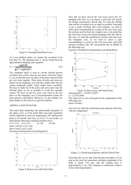
Figure 8. Uncompensated Root LocusAs it was defined earlier, we require the overshoot to beless than 5%. The damping ratio z, can be found from theapproximation damping ratio equation:log( 0.05)z = −(21)2( π2 + log(0.05) )The command 'sgrid' is used to overlay desired percentovershoot line on the close-up root locus. From the Figure8., we see that there are two pairs of the poles and zeros thatare very close together. These pairs of poles and zeros arealmost on the imaginary axis and they might make the bussystem marginally stable, which might cause a problem.We have to make all of the poles and zeros move into theleft-half plane as far as possible to avoid the unstablesystem. We have to put two zeros very close to the twopoles on the imaginary axis of uncompensated system forpole-and-zero cancellation. Moreover, we put another twopoles further on the real axis to get fast response.ADDING A NOTCH FILTERThe notch filter diminishes the unfavourable dynamics ofthe object. Let's se if the notch filter (two-lead controller)will be sufficient to meet our requirements. We shall put thepoles at 30 and 60, and zeros at 3±3.5i. To our m-file, weshall add the following command and then run it:z1=3+3.5i; z2=3-3.5i; p1=30; p2=60;numc=conv([1 z1],[1 z2]);denc=conv([1 p1],[1 p2]);rlocus(conv(nump,numc),conv(denp,denc))Now that we have moved the root locus across the 5%damping ratio line, we can choose a gain that will satisfythe design requirements. Recall that we want the settlingtime and the overshoot to be as small as possible. Generally,to get a small overshoot and a fast response, we need toselect gain corresponding to a point on the root locus nearthe real axis and far from the complex axis or the point thatthe root locus crosses the desired damping ratio line. But inthis case, we need the cancellation of poles and zeros nearthe imaginary axis, so we need to select a gaincorresponding to a point on the root locus near zeros andpercent overshoot line. We can perform this in Matlab inthe following way:[k,poles]=rlocfind(conv(nump,numc),conv(denp,denc))Figure 10. Root Locus with Notch Filterselected point = -2.9559+3.4307ik = 2.2755e+008The value of k we use as the gain for the compensator in thefollowing way:numc=k*numc;Now let's see what the closed-loop step response looks likewith the compensator:Figure 11. Closed-loop Response with the Notch FilterFigure 9. Root Locus with Notch FilterFrom this plot we see that when the bus encounters a 0.1mstep on the road, the maximum oscillation amplitude of itsbody is about 1.65 mm, and the settling time isapproximately 2 sec. This response is satisfactory relativeto the initial requirements.6