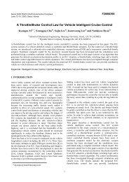
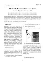
∗ mass distribution coefficient is approximately 1.Although the real characteristics <strong>of</strong> the suspension system(k1, b1) are non-linear, we have adopted constant values forthem in this paper which, without any significant error,enable the linearization <strong>of</strong> the model. The same has beendone for k2 <strong>and</strong> b2. The designations on Figure 1. have thefollowing meanings:∗ body mass (m1) = 2250 (285) kg;∗ suspension mass (m2) = 290 (60) kg;∗ spring constant <strong>of</strong> suspension system (k1) = 72000(25400) N/m;∗ spring constant <strong>of</strong> wheel <strong>and</strong> tyre (k2) = 450000(200000) N/m;∗ damping constant <strong>of</strong> suspension system (b1) = 315(1300) Ns/m;∗ damping constant <strong>of</strong> wheel <strong>and</strong> tyre (b2) = 13500 (700)Ns/m;∗control force (F a ) = force from the controller we aregoing to design.The data that we used during the simulation are for a bus<strong>and</strong> a passenger car (in the brackets). We have performedsimulations for both categories <strong>of</strong> vehicles (M 3 <strong>and</strong> M 1 -according to ECE Regulations), but have presented hereonly the results obtained for the bus. However, the adoptedconclusions also apply to the passenger car.BodyMass<strong>Suspension</strong>Massk 1Figure 1. - ¼ Vehicle ModelWhen the vehicle is experiencing any road disturbance, thebody should not have large oscillations, <strong>and</strong> the oscillationsshould dissipate quickly. This, at the same time, is ourprincipal task. Since the distance x 1 -W is very difficult tomeasure, <strong>and</strong> the deformation <strong>of</strong> the tyre x 2 -W is negligible,we will use the distance x 1 -x 2 instead <strong>of</strong> x 1 -W as the outputin our problem. The road disturbance W will be simulated<strong>by</strong> a step input. This step could represent the vehiclecoming out <strong>of</strong> a pothole. We want to design a feedbackcontroller so that the output x 1 -x 2 has an overshoot less than5% <strong>and</strong> a settling time shorter than 5 seconds. For example,when the vehicle runs onto a 10 cm high step, the body willoscillate within a range <strong>of</strong> ±5 mm <strong>and</strong> return to a smoothride within 5 seconds.MODELLING BY USING TRANSFER FUNCTIONk 2The assessment <strong>of</strong> the quality <strong>of</strong> automatic regulationsystem behaviour essentially boils down to estimating theerror between a predetermined value <strong>and</strong> the real value <strong>of</strong>the controlled variable. The knowing <strong>of</strong> this error at anypoint would give a complete information on the features <strong>of</strong>the observed system. Due to the diversity <strong>of</strong> the laws <strong>of</strong> theF ab 2b 1X 1X 2Wsystem's input change, which might occur in the normalwork regime, such an approach, based on estimation <strong>of</strong> thecurrent values <strong>of</strong> error, is inappropriate speaking from theaspect <strong>of</strong> practice. Therefore, it is preferable to make anestimation <strong>of</strong> the relevant system characteristics on thebasis <strong>of</strong> the features it manifests at its being disturbed <strong>by</strong>the typical input signals. With such an approach, the systemis being defined both in the stationary <strong>and</strong> transitional workregime. On the basis <strong>of</strong> Figure 1. <strong>and</strong> the Newton's Law, wecan obtain the following dynamic equations, whichrepresent the mathematical model <strong>of</strong> the dynamic system:m 1 x1 = −b1(x1 − x2)− k1(x1− x2)+ Fa(1)m2x2= b1(x1 − x2)+ k1(x1− x2)+ b2(W− x2)+(2)+ k 2(W− x2)− FaThe solving <strong>of</strong> these equations is, to a large extent,simplified <strong>by</strong> the application <strong>of</strong> Laplace transforms. Withthe help <strong>of</strong> these, we can immediately obtain the solutionfor the linear differential equations with constantcoefficients for the given initial conditions. The transformsprovide the representation <strong>of</strong> the system in the form <strong>of</strong> anappropriate block diagram. Although Laplace transformsmay not be the most ideal solution due to the possibility <strong>of</strong>complex algebra occurrence, the majority <strong>of</strong> procedures forthe synthesis <strong>and</strong> analysis <strong>of</strong> the automatic control system,more or less, relies on the application <strong>of</strong> LaplaceTransforms. This approach is not possible with linear nonstationarysystems, in which one or several parametreschange in time [4]. Let's assume that all the initialconditions are zeroes, so these equations represent thesituation when a wheel goes up a bump. The dynamicequations above can be expressed in a form <strong>of</strong> transferfunctions <strong>by</strong> taking Laplace Transform <strong>of</strong> the aboveequations. The derivation from above equations <strong>of</strong> theTransfer functions G 1 (s) <strong>and</strong> G 2 (s) <strong>of</strong> output, x 1 -x 2 , <strong>and</strong> twoinputs, F a <strong>and</strong> W, are as follows:M⎡ 2(m ⎤1s+ b1s+ k1)− (b1s+ k1)⎢⎥ *2⎢⎣− (b1s+ k1)m2s+ (b1+ b2)s+(k1+ k 2)⎥⎦(3)⎡X1(s)⎤ ⎡ Fa(s) ⎤* ⎢ ⎥ = ⎢⎥⎣X2(s)⎦ ⎣(b2s+k 2)W(s)− Fa(s) ⎦2∆ = det[ M]= (m1s+ b1s+ k1) *(4)22* (m2s+ (b1+ b2)s+(k1+ k 2))− (b1s+ k1)Then, we find the inverse <strong>of</strong> the matrix A <strong>and</strong> multiply withinputs F a (s) <strong>and</strong> W(s) on the right h<strong>and</strong> side as thefollowing:⎡m2s2+ 2⎤⎢b 1 b 2 s + (b 1 k 2 + b 2 k 1 )s+k 1 k 2 ⎥⎡X1(s)⎤ 1 ⎢+b 2 s+k 2⎥⎢ ⎥ = **X2(s)⎢m3(m b2 ⎥⎣ ⎦ ∆⎢ 2 1 b 2 s + 1 k 2 + 1 b 2 )s +− m 1 s⎥⎢(b1k2 b2k1)s⎥⎣+ + + k1k2 ⎦⎡F a (s) ⎤* ⎢ ⎥(5)⎣W(s)⎦When we want to consider input F a (s) only, we set W(s)=0.Thus we get the transfer function G 1 (s) as the following:2X1(s)− X 2(s)(m1+ m2)s+ b2s+k 2G 1(s)==(6)Fa(s)∆2
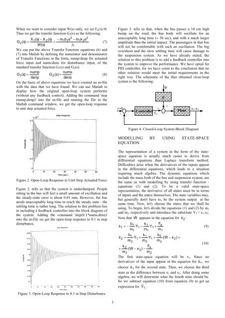
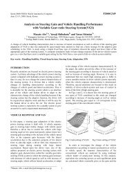
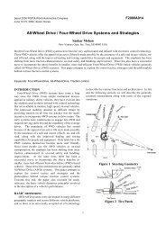
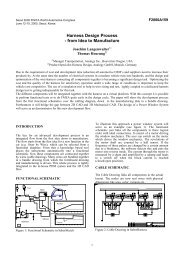
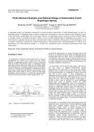
When we want to consider input W(s) only, we set F a (s)=0.Thus we get the transfer function G 2 (s) as the following:3 2X1(s)− X 2(s)− m1b2s− m1k2sG 2(s)==(7)W(s)∆We can put the above Transfer Function equations (6) <strong>and</strong>(7) into <strong>Matlab</strong> <strong>by</strong> defining the numerator <strong>and</strong> denominator<strong>of</strong> Transfer Functions in the form, nump/denp for actuatedforce input <strong>and</strong> nums/dens for disturbance input, <strong>of</strong> thest<strong>and</strong>ard transfer function G 1 (s) <strong>and</strong> G 2 (s):numpnumsG1 (s) = G2(s)=(8)denpdensOn the basis <strong>of</strong> above equations we have created an m-filewith the data that we have found. We can use <strong>Matlab</strong> todisplay how the original open-loop system performs(without any feedback control). Adding the comm<strong>and</strong> 'step(nump,denp)' into the m-file <strong>and</strong> running the file in the<strong>Matlab</strong> comm<strong>and</strong> window, we get the open-loop responseto unit step actuated force.Figure 3. tells us that, when the bus passes a 10 cm highbump on the road, the bus body will oscillate for anunacceptably long time (≈ 50 sec), <strong>and</strong> with a much largeramplitude than the initial impact. The passengers in that buswill not be comfortable with such an oscillation. The bigovershoot <strong>and</strong> the slow settling time will cause damage tothe suspension system. As we have already stated, thesolution to this problem is to add a feedback controller intothe system to improve the performance. We have opted forPID controller, for we have come to the conclusion that noother solution would meet the initial requirements in theright way. The schematic <strong>of</strong> the thus obtained close-loopsystem is the following:r=0 ++ControllerPlantx -x 1 2+ F-aFWFigure 4. Closed-Loop <strong>System</strong> Block DiagramMODELLING BY USING STATE-SPACEEQUATIONFigure 2. Open-Loop Response to Unit Step Actuated ForceFigure 2. tells us that the system is underdumped. Peoplesitting in the bus will feel a small amount <strong>of</strong> oscillation <strong>and</strong>the steady-state error is about 0.01 mm. However, the busneeds unacceptably long time to reach the steady state - thesettling time is rather long. The solution to this problem liesin including a feedback controller into the block diagram <strong>of</strong>the system. Adding the comm<strong>and</strong> 'step(0.1*nums,dens)'into the m-file we get the open-loop response to 0.1 m stepdisturbance.Figure 3. Open-Loop Response to 0.1 m Step DisturbanceThe representation <strong>of</strong> a system in the form <strong>of</strong> the statespaceequation is usually much easier to derive fromdifferential equations than Laplace transform method.Difficulties arise when the derivatives <strong>of</strong> the inputs appearin the differential equations, which leads to a situationrequiring much algebra. The dynamic equations whichinclude the mass both <strong>of</strong> the bus <strong>and</strong> suspension system, arethe same as with modelling <strong>by</strong> using transfer function -equations (1) <strong>and</strong> (2). To be a valid state-spacerepresentation, the derivative <strong>of</strong> all states must be in terms<strong>of</strong> inputs <strong>and</strong> the states themselves. The state variables may,but generally don't have to, be the system output at thesame time. Now, let's choose the states that we shall beusing. To begin, let's divide the equations (1) <strong>and</strong> (2) <strong>by</strong> m 1<strong>and</strong> m 2 , respectively <strong>and</strong> introduce the substitute Y 1 = x 1 -x 2 .Note that W appears in the equation for x 2 :b1k1F ax 1 = − Y1 − Y1+(9)m1m1m1b1k1b2x2= Y1 + Y1+ (W− x2)+m2m2m2(10)k 2Fa+ (W − x2)−m2m2The first state-space equation will be x 1 . Since noderivatives <strong>of</strong> the input appear in the equation for x 1 , wechoose x 1 for the second state. Then, we choose the thirdstate as the difference between x 1 <strong>and</strong> x 2 . After doing somealgebra, we will determine what the fourth state should be.So we subtract equation (10) from equation (9) to get anexpression for Y 1 :3