Phase diagrams of a two-dimensional Heisenberg antiferromagnet ...

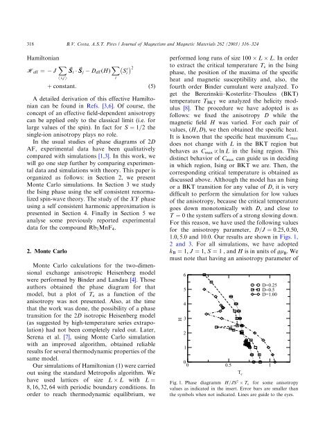
318B.V. Costa, A.S.T. Pires / Journal of Magnetism and Magnetic Materials 262 (2003) 316–324HamiltonianH eff ¼J X /i;jSþ constant:~S i ~ S j D eff ðHÞ X iSiz 2ð5ÞA detailed derivation of this effective Hamiltoniancan be found in Refs. [3,6]. Of course, theconcept of an effective field-dependent anisotropycan be applied only to the classical limit (i.e. forlarge values of the spin). In fact for S ¼ 1=2 thesingle-ion anisotropy plays no role.In the usual studies of phase diagrams of 2DAF, experimental data have been qualitativelycompared with simulations [1,3]. In this work, wewill go one step further by comparing experimentaldata and simulations with theory. This paper isorganized as follows: in Section 2, we presentMonte Carlo simulations. In Section 3 we studythe Ising phase using the self consistent renormalizedspin-wave theory. The study of the XY phaseusing a self consistent harmonic approximation ispresented in Section 4. Finally in Section 5 weanalyse some previously reported experimentaldata for the compound Rb 2 MnF 4 :2. Monte CarloMonte Carlo calculations for the two-dimensionalexchange anisotropic Heisenberg modelwere performed by Binder and Landau [4]. Thoseauthors obtained the phase diagram for thatmodel, but a plot of T c as a function of theanisotropy was not presented. Also, at the timethat the work was done, the possibility of a phasetransition for the 2D isotropic Heisenberg model(as suggested by high-temperature series extrapolation)had not been completely ruled out. Later,Serena et al. [7], using Monte Carlo simulationwith an improved algorithm, obtained reliableresults for several thermodynamic properties of thesame model.Our simulations of Hamiltonian (1) were carriedout using the standard Metropolis algorithm. Wehave used lattices of size L L with L ¼8; 16; 32; 64 with periodic boundary conditions. Inorder to reach thermodynamic equilibrium, weperformed long runs of size 100 L L: In orderto extract the critical temperature T c in the Isingphase, the position of the maxima of the specificheat and magnetic susceptibility and, also, thefourth order Binder cumulant were analyzed. Toget the Berezinskii–Kosterlitz–Thouless (BKT)temperature T BKT we analyzed the helicity modulus[8]. The procedure we have adopted is asfollows: we fixed the anisotropy D while themagnetic field H was varied. For each pair ofvalues, ðH; DÞ; we then obtained the specific heat.It is known that the specific heat maximum C maxdoes not change with L in the BKT region butbehaves as C max pln L in the Ising region. Thisdistinct behavior of C max can guide us in decidingin which region, Ising or BKT we are. Then, thecorresponding critical temperature is obtained asdiscussed above. Although the model has an Isingor a BKT transition for any value of D; it is verydifficult to perform the simulation for low valuesof the anisotropy, because the critical temperaturegoes down monotonically with D; and close toT ¼ 0 the system suffers of a strong slowing down.For this reason, we have used the following valuesfor the anisotropy parameter, D=J ¼ 0:25; 0:50;1:0; 5:0 and 10:0: Our results are shown in Figs. 1,2 and 3. For all simulations, we have adoptedk B ¼ 1; J ¼ 1; S ¼ 1 , and H is in units of gm B : Wemust note that having an anisotropy parameter ofH65432100 0.5 1T cD=0.25D=0.5D=1.00Fig. 1. Phase diagramm H=JS 2 T c for some anisotropyvalues as indicated in the insert. Error bars are smaller thanthe symbols when not indicated. Lines are guide to the eyes.