Phase diagrams of a two-dimensional Heisenberg antiferromagnet ...

More documents

Recommendations

Info

B.V. Costa, A.S.T. Pires / Journal of Magnetism and Magnetic Materials 262 (2003) 316–324 321pairs. This latter mechanism is responsible for ashift in the transition temperature [13]. AtT BKTrenormalization group analysis [14] shows that thestiffness should exhibit a universal jump given by2T BKT =p: The BKT temperature for our model canthen be determined by the crossing between therðTÞ curve, calculated using Eq. (18) and the lineg ¼ 2T=p: Our calculation for the XY region isalso presented in Fig. 2. The two phase boundariesmeet at T ¼ 0 for H ¼ H sf ; with a horizontaltangent. At low temperatures, the two critical linesare so close to each other, that they cannot bedistinguished from a single spin-flop line. In theXY region, an applied field is not really equivalentto an anisotropy: increasing the field would leadthe spins to tilt out of the XY plane while a trueanisotropy would force the spins to lie in the XYplane. The SCHA works reasonably well for theanisotropic easy-plane Heisenberg model [11–15],and the effect of the tilting out of the plane wastaken into account by the sin 2 y 0 term in Eq. (18).However, even so, the quantitative agreement isgood only for the regions HBH sf and HBH c ; forother values of H; the agreement is not so good. Itseems, then, that the reduction of the spin in-planecomponent was not completely taken into accountin our calculation and a more elaborated theoryshould be developed.approximately given by [1]pH sf ¼ffiffiffiffiffiffiffiffiffiffiffiffiffiffiffiffiffiffiffiffiffiffiffiffiffiffiffiffiffi28:09 þ 0:23T; ð22Þwhere T is the temperature in Kelvin, and H isgiven in Tesla. For a 2D system, described byHamiltonian (1), we would have just a bicriticalpoint at T ¼ 0: A line of zero anisotropy impliesthe existence of long range order for H ¼ H sf : Thecomparison of our theoretical calculation with theexperiments of Ref. [1] is shown in Figs. 4 and 5.Aquantum SCHA for an easy-plane model with S ¼5=2 gives results similar to the ones using theclassical approximation [18] and, therefore, in theXY region we are allowed to use the simplerclassical approach presented in Section 4. Thehigher-field phase boundary can be fitted reasonablywell by our theory. In Fig. 4 we use the valueD ¼ 0:148 K; and in Fig. 5 we use a temperaturedependent value obtained using Eq. (22). For H7655. Rb 2 MnF 4A material which is particularly close to classicaltwo-dimensional models seems to be Rb 2 MnF 4which has spin S ¼ 5=2 [16]. At zero field thiscompound is a weakly Ising antiferromagnet withJ ¼ 7:31 K: The principal spin anisotropy is anuniaxial magnetic interaction with gm B H A ¼0:371 K evaluated at a temperature of T ¼ 4:2K;along the z-axis perpendicular to the magneticplane. Using the relationDS 2 ¼ gm B H A S;we find D ¼ 0:148 K: The magnetic ordering hasbeen described by Birgeneau et al. [17]. In zerofield, the system undergoes a transition to a 2Dmagnetically ordered structure at 38:4K: The lineof zero anisotropy was experimentally found to beField (T)432100 10 20 30 40Temperature (K)Fig. 4. Phase diagram for Rb 2 MnF 4 in an external magneticfield perpendicular to the magnetic planes. The experimentaldata (circles) are from Ref. [1]. Squares represent Greenfunction calculation in the Ising region and SCHA in the XYregion. Diamonds are the SCR calculation.
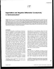
322B.V. Costa, A.S.T. Pires / Journal of Magnetism and Magnetic Materials 262 (2003) 316–324Field (T)7654This technique has been used by Dalton and Wood[20] and Reinehr Figueiredo [21] to study theferromagnet with exchange anisotropy. The retardedGreen function for Heisenberg operators Aand B is defined asG A;B ðtÞ iyðtÞ/½AðtÞ; Bð0ÞŠS; ð23Þin which yðtÞ is the step function equal to 1 fort > 0; 0 for to0: The equation of motion for thetime-Fourier transformation of G AB ðtÞ given by0A; BT ¼ 1 Z þNG AB ðtÞe iot dt;2pisNo0A; BT ¼ 12p /½A; BŠS þ 0½AðtÞ; HŠ; Bð0ÞT; ð24Þ30 10 20 30 40Temperature (K)where H is the Hamiltonian of the system. ForHamiltonian (1) we findFig. 5. Phase diagram for Rb 2 MnF 4 in an external magneticfield perpendicular to the magnetic planes.The experimentaldata (circles) are from Ref. [1]. Squares are Green functioncalculations taking into account the interplanar coupling.Diamonds are Green function calculations in the Ising regionand SCHA in the XY region, with a temperature dependentanisotropy.o0Sn þ ; S m T ¼ 1 p /Sz n Sd m;nþ J X 0S þ nþd Sz n ; S m Td0Sn z Sþ nþd ; S m T0Snþd z Sþ n ; S mTþ D eff 0Sn þ Sz n ; S m Tþ 0Sn z Sþ n ; S m T :ð25Þup to 7 T, the effective anisotropy formulation isexpected to work since, in this case, H c E65 T: Inthe Ising phase, for a more precise comparisonwith the experimental data, we performed aquantum SCR calculation. We obtain the quantumSCR expression by replacing T=E q byðexpðE q =TÞ 1Þ 1 in Eqs. (7) and (8) [9]. However,now, due to the exponential term, the numericalsolution of the self consistent equations must beperformed in a very carefull way since the accuracydecreases with decreasing temperature. In Fig. 4we also show the theoretical calculation using theSCR technique. The results are not very differentfrom the ones obtained using the Green functiontechnique described below which is a moreconvenient approach and easier to calculate [19].In order to solve Eq. (25) we use the random-phaseapproximation to decouple the higher order Greenfunction, this is0S z n Sþ m ; S j T ¼ /S z n S0Sþ m ; S j T;to obtaino0S þ n ; S m T¼ 1 p /Sz n Sd m;n þ 2J/Sn z S X 0S þ nþd ; S m T þ 0Sþ n ; S m Tdþ 2D eff /S z n S0Sþ n ; S m T:ð26Þð27ÞWe remark that in the limit J-0 (and H ¼ 0) wehave /S z S-0 even if Da0; and the above
Page 1 and 2: Journal of Magnetism and Magnetic M
Page 3 and 4: 318B.V. Costa, A.S.T. Pires / Journ
Page 5: 320B.V. Costa, A.S.T. Pires / Journ
Page 9: 324B.V. Costa, A.S.T. Pires / Journ

Phase diagrams of a two-dimensional Heisenberg antiferromagnet ...

You also want an ePaper? Increase the reach of your titles

Delete template?

Save as template?