DSP Formulation of a Finite Difference Method for Room Acoustics ...

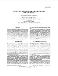
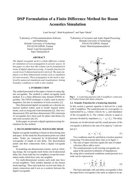
DSP Formulation of a Finite Difference Method for RoomAcoustics SimulationLauri Savioja 1 , Matti Karjalainen 2 , and Tapio Takala 11 Laboratory of Telecommunications Softwareand MultimediaHelsinki University of TechnologyFIN-02150 ESPOO, FinlandEmail: Lauri.Savioja@hut.fiTapio.Takala@hut.fiABSTRACTThe digital waveguide mesh is a finite difference schemefor simulation of wave propagation in acoustic spaces. Inthis paper we show how this scheme can be formulated interms of digital signal processing. A transfer function fora node in an N-dimensional mesh is derived. The main emphasisis in three-dimensional systems such as simulationof room acoustics. Wave propagation in the mesh is analyzedby numerical simulations and visualizations. Settingboundary conditions to walls is also studied.1. INTRODUCTIONThe method presented in this paper is based on using digitalwaveguides. The method is called waveguide meshmethod. It is a finite difference time domain (FDTD) algorithm.The FDTD technique is widely used in electromagnetics,but also in simulation of room acoustics [1].One-dimensional digital waveguides are a discrete numericalmethod widely used to model musical instruments,such as string and wind instruments [2]. Also twodimensional(2D) and three-dimensional (3D) extensionsof waveguides have been used for plates and drums [3],and room acoustics [4], [5].In this paper we present a digital signal processing formulationfor this method.2. MULTI-DIMENSIONAL WAVEGUIDE MESHDigital waveguide modeling is based on discretizing timeand space. In this study the discretization points are callednodes. Nodes are connected by bi-directional digitalwaveguides of length of unit delay. The discretizationpoints and their connections form a digital waveguidemesh.In modeling one-dimensional systems, such as vibratingstrings, the waveguide mesh forms one bi-directionaldelay line. Each node has two neighbors except the terminationnodes which have only one neighbor.For multi-dimensional systems each node may haveseveral neighbors. Their number depends on the chosenmesh topology. Thus each node has several unit delay elementconnections and it acts as a scatterer between thedigital waveguides.2 Laboratory of Acoustics and Audio Signal ProcessingHelsinki University of TechnologyFIN-02150 ESPOO, FinlandEmail: Matti.Karjalainen@hut.fip + 1,oppp 1,oppp - 1,oppp 2,oppp - 1 p + p+ p N,opp N,opp1p - N p - N,oppp + Np 3,oppp 4,opp4...NFig 1. A scattering junction with N neighbors connectedby bi-directional unit delay elements.2.1. Transfer Function for a Scattering JunctionIn this section a general equation is derived for a nodewith N neighbors. The sound pressure in a waveguide i isrepresented by p i , volume velocity by v i , and impedanceof the waveguide by Z i . The volume velocity is equal topressure divided by impedance ( v i= p i⁄ Z i). The delayelements are bi-directional and the sound pressure of thewaveguide is defined as the sum of its input (p + ) and output(p - )+p i= p i+ p ī(1)Two conditions must be satisfied at a lossless junctionconnecting N bi-directional delay lines as in figure 1:1. The sum of input velocities equals the sum of outputvelocities (flows add to zero)2. The sound pressures in all crossing waveguides areequal at the junction (continuity of impedances).By using above mentioned conditions sound pressure at anode can be expressed asN +p Ni 1p = 2 ∑ ----- ⁄Z∑ ----(2)iZi = 1 i = 1 iThe basic principle with unit-delay waveguides is thatthe input from a waveguide is the same as output in its op-

posite end one time step before. This can be expressed asthe equation+p iz – 1 -= p i,opp(3)-where p i,opppresents output at opposite end of thewaveguide i. By using equations (1) and (3) the soundpressure in a node takes the following formNz – 1Np i,oppz – 1 +p i, opp2 ∑ ------------------------ 2Z∑ ------------------------iZpi = 1i= --------------------------------------- – ---------------------------------------i = 1(4)NN11∑ ----Z∑ ----iZi = 1i = 1 iBy applying once again the same equations we get an expressionfor sound pressureN p iopp ,2 ∑ ---------------p z – 1 Zi = 1 i= ------------------------------ – z – 2 p(5)N1∑ ----Zi = 1 iEquation (5) can be expressed also in form of a transferfunctionz – 1 N p Ni, opp 1⋅ 2 ∑ --------------- ⁄Z∑ ----iZpi = 1i= ----------------------------------------------------------------i = 1(6)1 + z – 2In a usual case the medium is homogenous and impedancesin all waveguides are equal and equation (6) can bereduced to the formz – 1 2 N⋅ --- N∑ p i,oppp = ---------------------------------------------i = 1(7)1 + z – 2Verbal description of equation (7) is that the sound pressurein a node is two times the average of its neighborssubtracted by its own value two time units ago. This expressionis independent of the dimensionality of the system.Only the number of neighbors is relevant.2.2. Mesh ExcitationExciting the mesh must be done so that none of the equations(1)-(5) is violated. If we want to create an excitationof value I in a homogenous mesh at a node with N neighbors,we set the incoming sound pressure to allwaveguides connected to it. Using equation (2) the valuefor sound pressure is found to be+ Ip i= -- ∀i= 1…N(8)2To keep the equation (3) satisfied the history of neighborshas to be updated also, since the outgoing sound pressuresin opposite ends of waveguides at one time stepbefore excitation must equal to I/2. Because there are noother outputs, the sum of output signals is also I/2, which1D3D2DFig 2. Example structures of rectilinear 1D, 2D and 3Dmeshes.is the same as the sum of input signals. By using equation(2) again we come to the result that all the neighbor nodesmust have value I/N at one time step before excitation.3. MESH STRUCTUREThere are different topologies which may be used to constructa digital waveguide mesh. The only restriction isthat all the delay-elements connecting nodes must be ofequal length. If there are waveguides of different lengths,the equation (5) is no more valid. Instead, equation (4) canbe used, z – 1– xis replaced with z i, and x represents the delaylength of waveguide i.The requirement of equal length waveguides is satisfiedby any regular space decomposition method. It meansthat the atomic tiles of decomposition are polytopeswhose sides are of equal length [6]. In this study we concentrateon rectilinear meshes, since they are computationallyefficient and easy to construct. Some hexagonal,triangular and tetrahedral structures both in 2- and 3-dimensionalsystems are presented in [7] and [8].An N-dimensional rectilinear waveguide mesh is aregular array of digital 1-D waveguides arranged alongeach perpendicular dimension, interconnected at theircrossings. In figure 2 there are examples of meshes of differentdimensionalities.In an N-dimensional rectilinear mesh each node insidethe mesh has exactly 2*N neighbors. Nodes on the boundarieshave only one neighbor. Due to this arrangement theboundaries can be terminated the same way as in digital1D waveguides.3.1. Sampling Frequency of a Rectilinear MeshDistance between mesh nodes together with the mesh topologydetermines the sampling rate of the mesh. In a onedimensionalsystem waves propagate one unit distance inone time unit since the waveguide mesh is constructed ofunit-delays.In a multi-dimensional rectilinear mesh effective wavepropagation speed is found at the diagonal direction. In anN-dimensional system one diagonal movement, correspondingto distance of N unit distances, requires N unitdelays. Thus the update frequency of a rectilinear N-dimensionalmesh is

c Nf = ----------(9)dxwhere c represents the speed of sound in the medium anddx is the unit distance between two nodes. For example inair c ≈ 340m ⁄ s, and if a 3D mesh is discretized withspacing of 5 cm, the update frequency will be ca. 12 kHz.3.2. Rectilinear 3D Waveguide MeshFor studying the behavior of rectilinear 3D waveguidemesh we have made numerical simulations. Equation (7)can be expressed also as a difference scheme1pn ( ) = -- (10)3∑ p ( i, oppn – 1 ) – pn ( – 2)iwhere p i,opp are the axial 3D neighbors of a node, and nrepresents time. This scheme is equivalent to the differenceequation derived from the wave equation by discretizingtime and space with forward-time-center-spacemethod. Simulations are made in a mesh with 3 cm discretizationgrid, corresponding to sampling frequency ofca. 20 kHz.In figure 3 the magnitude responses registered at differentdistances along a 2D diagonal of the mesh areshown. The figure shows that doubling the distance fromthe sound source attenuates signal 6dB like it should do ina real 3D environment.The shape of the transfer function is due to the natureof excitation. The source is point like and its impedance isfrequency dependent so that low frequencies are attenuated.The magnitude response is symmetrical to half of theNyquist frequency and for that reason only the first half isshown.Figure 4 presents two impulse responses in time domain.The first one is registered in axial and the second in3D diagonal direction. The responses are quite differentfrom each other. The diagonal response has ideal attenuationslope, but the axial response is distorted. The reasonfor this is that the mesh is anisotropic. Wave propagationcharacteristics are direction dependent.Sound pressureSound pressure210−1Impulse response (axial)−20 100 200 300 400 500 600 700Time (in samples)Impulse response (3D−diagonal)420−2−40 100 200 300 400 500 600 700Time (in samples)Fig 4. Impulse responses to axial and 3D-diagonaldirections at the same distance from the sound source.Figure 5 shows the effect of mesh anisotropy to magnituderesponse. The difference is largest between axial(az=0˚, el=0˚) and diagonal (az=45˚,el=45˚) propagation.Signal has attenuated in axial direction at higher frequencies.Up to one fifth of the Nyquist frequency the magnituderesponse to all directions is within 2 dB.Figure 6 shows the dispersion characteristics of themesh. In the figure there are group delays to three differentdirections. Both the 2D and 3D diagonals introduce noobvious dispersion while in axial direction the dispersionis remarkable above one fifth of the Nyquist frequency.Considering both the magnitude and phase the validfrequency range for simulations is from DC to about onetenth of the sampling frequency.4. BOUNDARY CONDITIONSThe most straightforward way to set boundary conditionsis the mesh structure where each boundary node has onlyone neighbor. There are also other possible ways, but inthis study we concentrate on the 1D termination. If wehave a boundary with reflection coefficient r, the transferfunction for the boundary node is403020Magnitude Response (dB)20100−10Distance from0.1m0.25m0.5mMagnitude Response (dB)100−10−20az=0°, el=0°az=45°, el=0°az=45°, el=45°Azimuth and−20Sound Source1m2m−30az=30°, el=0°az=30°, el=30°elevation angles0 0.05 0.1 0.15 0.2 0.25Normalized Frequency (Nyquist == 0.5)Fig 3. Magnitude response registered from various distancesat diagonal direction.0 0.05 0.1 0.15 0.2 0.25Normalized Frequency (Nyquist == 0.5)Fig 5. Magnitude response from constant distance tovarious angles.

600AxialGroup delays (in samples)40020000 0.05 0.1 0.15 0.2 0.256004002002−D Diagonal00 0.05 0.1 0.15 0.2 0.256004002003−D Diagonal00 0.05 0.1 0.15 0.2 0.25Normalized frequency (Nyquist == 0.5)Fig 6. Group delays in three different directions, axial,2D diagonal and 3D diagonal.( 1 + r) ⋅ z – 1 poppp = -----------------------------------------(11)1 + rz – 2This result is found by using equation (4) and setting+p wall= 0 , since there is no input from inside the wall.In addition the following relation between impedanceZchange and reflection factor is used: r 2 – Z= ------------------ 1. Equation(11) can also be expressed as a difference equationZ 2 + Z 1pn ( ) = ( 1 + r) ⋅ p opp( n – 1)– r ⋅ p( n–2)(12)where p is the boundary node and p opp is its neighbor. Ingeneral the boundary condition can be replaced by anydigital filter.Figure 7 shows behaviour of some simple boundaryconditions. The model consists of three rooms constructedof different materials. The first figure shows the roomconfiguration, excitation shape and first order phase preservingreflection from the ceiling. In the second one thereare phase reversing reflections from the walls. The wallsseparating rooms are anechoic.5. SUMMARY AND FUTURE WORKIn this paper we have shown that finite difference time domainmethod can also be formulated in terms of digitalsignal processing. The study is based on digitalwaveguides.In the future we are going to make this algorithm tobetter suit real room acoustic problems. This includes adetailed study on boundary conditions and also on couplingof different sound propagation mediums. To enhancedispersion characteristics various interpolationtechniques are under study, and some results are describedin a companion paper [9].Fig 7. Visualization of simulation, excitation andfirst order reflection (above), wall reflections (below).REFERENCES[1] D. Botteldooren, “Finite-difference time domain simulationof low-frequency room acoustic problems,” J.Acoust. Soc. Am., vol. 98, no. 6, pp. 3392-3308, 1995.[2] J. Smith, “Physical modeling using digitalwaveguides,” Computer Music Journal, vol. 16, no.4, pp. 75-87, Winter 1992.[3] S. Van Duyne and J. Smith, “Physical modeling withthe 2-D digital waveguide mesh,” In Proc. 1993 Int.Computer Music Conf., Tokyo, Sept. 10-15, 1993, pp.40-47.[4] L. Savioja, J. Backman, A. Järvinen, and T. Takala,“Waveguide mesh method for low-frequency simulationof room acoustics,” In Proc. 15th Int. Congresson Acoustics (ICA’95), Trondheim, Norway, June 26-30, 1995, vol. 2, pp. 637-640.[5] L. Savioja, A. Järvinen, K. Melkas, and K. Saarinen,“Determination of the low-frequency behaviour of anIEC listening room,” In Proc. Nordic AcousticalMeeting (NAM’96), Helsinki, Finland, June 12-14,1996, pp 55-58.[6] H. Samet, The Design and Analysis of Spatial DataStructures, Addison-Wesley, 1990.[7] S. Van Duyne and J. Smith, “The tetrahedral digitalwaveguide mesh”, In Proc. 1995 IEEE ASSP Workshopon Applications of Signal Proc. to Audio andAcoustics, New Paltz, NY, Oct. 1995.[8] S. Van Duyne and J. Smith, “The 3D tetrahedral digitalwaveguide mesh with musical applications”, InProc. 1996 Int. Computer Music Conf., Hong Kong,Aug. 19-24, 1996, pp. 9-16.[9] L. Savioja and V. Välimäki, “The bilinearly deinterpolatedwaveguide mesh,” In Proc. NORSIG’96 IEEENordic Signal Processing Symposium, Espoo, Finland,Sept. 24-27, 1996.