The sonification of numerical fluid flow simulations

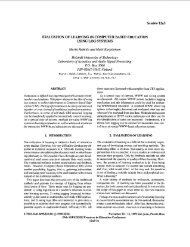
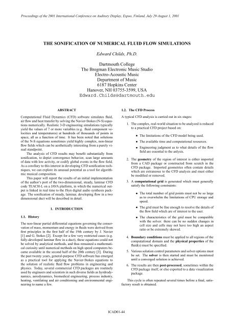
Proceedings of the 2001 International Conference on Auditory Display, Espoo, Finland, July 29-August 1, 20012. PHYSICAL AND MATHEMATICAL BASIS OF THECFD SOLVER2.1. The Governing EquationsIn the case of steady, two-dimensional flow, the continuity (conservationof mass) equation is:Ü´Ùµ · ´Úµ ¼ (1)Ýwhere is the local fluid density (kg/m ¿ ), Ù and Ú are the localfluid velocities (m/s) and Ü and Ý (m), correspond to the cartesiancoordinate system.For incompressible flow, the momentum equations are for theÜ direction:Ù Ù Ù ·ÚÜ Ý ÔÜ · Ü´¾ ÙÜ µ· Ù ´Ý Ý · Ú ℄µ (2)Üand for the Ý direction:Figure 2: Vectorsit uses are iterative by nature, and generate numbers that evolveover time. There is therefore a potential for CFD to generate livemusical compositions.1.5. Scope of Present WorkThis paper will focus on the real-time sonification of Stage 5 (solution)of the CFD process.An academic CFD research code TEACH-L [8], originallywritten in FORTRAN, was ported by the author to Java in orderto make use of JSyn [9], a digital audio synthesis package.JSyn (Java Synthesis) is a Java API (application programminginterface), which provides several classes of objects that can createand modify sound. A fast DSP synthesis package written inC lies beneath JSyn’s hood. All Java synthesis calls are passedtransparently to the C engine.TEACH-L solves the steady, laminar equations of the conservationof mass, momentum (Navier-Stokes) and energy on a twodimensional,cartesian grid, using a hybrid differencing sheme andthe SIMPLE (Semi-Implicit Method for Pressure-Linked Equations)algorithm [10] to correct the pressure field. The algebraicequations are solved line-by-line (LBL), using the tri-diagonal matrixalgorithm (TDMA). The TEACH-L code is extremely compact.There is no user-interface. To set up the geometry, grid,boundary conditions, and physical properties, the user must writeher own subroutines using the templates provided. This structurewas retained in the Java port, so that TEACH-L consists of a CFDAPI.The compactness of TEACH-L, together with the flexibility ofthe JSyn API, afforded a reasonable implementation on a MacintoshG3 Powerbook, providing a tool for the in-depth explorationof various sonification strategies for a CFD solver.In the following sections, the physical and mathematical basisof TEACH-L will be presented. One sonification strategy will beexplored, followed by results and conclusions.Ù Ú Ú · ÚÜ Ý ÔÝ ·Ü´ ÚÜ · ÙÝ ℄µ · Ý´¾ÚÝ µ(3)where is the acceleration due to gravity (m/s ¾ ), Ô is the fluidstatic pressure (Pa) and is the fluid dynamic viscosity (kg/ms).The energy conservation equation for the fluid, neglecting viscousdissipation and compression heating, is: Ô´Ù ØÜ · Ú ØÝ µÜ´ ØÜ µ·ÝØ ´ µ (4)Ýwhere Ô is the fluid specific heat at constant pressure (J/kg K), is the fluid thermal conductivity (W/m K), and Ø is the fluid staticpressure (K).2.2. DiscretizationTo solve the non-linear partial differential equations from the previoussection, it is necessary to impose a grid on the flow domainof interest, see Fig. 3. In TEACH-L, discrete values of fluid velocities,properties, pressure and temperature, are stored at each gridpoint (the intersection of two grid lines). To obtain a matrix of algebraicequations, a control volume is constructed (shaded area inthe figure) whose boundaries (shown by dashed lines) lie midwaybetween grid points È and its neighbors Æ, Ë, , Ï . A complexprocess of formal integration of the differential equations over thecontrol volume, followed by interpolation schemes to determineflow quantities at the control volume boundaries (Ò, ×, , Û) inFig. 3, finally yield a set of algebraic equations for each grid pointÈ [11]:´ È µ È (5)where the subscript on È , and refers to a summation overneighbor nodes Æ, Ë, and Ï , is a general symbol for thequantity being solved for (Ù, Ú or Ø), È , etc. are the combinedconvection-diffusion coefficients (obtained from integration andinterpolation), and and are, respectively, the implicit andexplicit source terms (and generally represent the force(s) whichdrive the flow, e.g. a pressure difference).ICAD01-46

Proceedings of the 2001 International Conference on Auditory Display, Espoo, Finland, July 29-August 1, 2001only one line at a time is solved, quantities on other lines are consideredto be “known”. Thus, a smaller Ò ¢ Ò tri-diagonal matrixresults, where Ò is the number of nodes in the direction. Thesolver starts at the first -index line in the solution domain, and“sweeps” from left to right.Because the partial differential equations are non-linear, theresulting algebraic matrix equations will be also, that is, the convection-diffusioncoefficients È , etc. will themselves be functionsof the ’s. An iterative solution is thus required, as follows:1. The coefficients for Eq.(5) in which Ù are formed, andthe current global “error” or “residual” is calculated. Thematrix of coefficients is solved by LBL and new values of Ù are obtained.2. The same is done for Ú and Ø.3. A “pressure correction” equation, derived from the massconservation equation is solved in a similar manner, the valuesof pressure at each note are updated [10].4. The global errors calculated in each of the above steps arethen all compared to a set of target values. If these errorsfall below the target, the solution has converged and the calculationstops. Otherwise, the calculation resumes at step 1.2.4. Solution Control Parameters2.3. SolutionFigure 3: Control VolumeEquation (5) must be written at each node where the value of È isrequired; doing so will generate an Æ ¢ Æ matrix of simultaneousequations, where Æ is the number of nodes in the solution domain.It is usually impractical to invert this matrix directly, so instead aline-by-line (LBL) scheme is used, see Fig. 4. In the LBL scheme,There are two sets of parameters which are set by the user to controlthe progress of the solution, the underrelaxation factors andthe sweep controls. In an iterative, numerical solution, underrelaxationslows the rate of change of a variable from one iterationto the next. Underrelaxation is necessary for numerical stabilityand to avoid divergence of the solution. Sweep controls for eachvariable are set to control the number of times, per iteration, theLBL procedure is applied to the coefficient matrix. The greater thenumber of sweeps, the better the matrix inversion at a particulariteration (but the greater the amount of CPU time required.)3. DUCT FLOW EXAMPLEAs an example of a solver sonification, the simple problem ofsteady, laminar, two-dimensional developing flow in a planar ductwill be considered (see Fig. 5). In this flow situation, fluid entersat the left with a uniform velocity profile, which develops, asthe fluid reaches the end of the duct on the right, into a parabolicprofile which is characteristic of “fully-developed” flow, Eq. 6:µ = 1.0 kg/msρ = 1.0 kg/m^3Uin = 1.0 m/s0.5 mFigure 4: Line-By-Line Scheme1.0 mFigure 5: Developing Flow in a 2D DuctÙ ¿ ¾Ý¾ÙÑ´½ µ (6)¾ where ÙÑ is the average velocity (in this case, 1 m/s), is theheight (in this case 0.5 m) and Ý ¼at the centerline of the duct.ICAD01-47

Proceedings of the 2001 International Conference on Auditory Display, Espoo, Finland, July 29-August 1, 2001When the flow is fully developed, the transverse velocity componentÚ vanishes, and the pressure Ô changes only linearly with Ü:¡Ô ½¾ÙÑ¡Ü ¾ (7)which gives the pressure drop ¡Ô over some Ü-direction length¡Ü, and where the viscosity is in this case 1 kg/ms.A coarse ¢ evenly spaced grid was used, yielding a total of ¢ ¾internal or “live” cells at which the values of Ù, Ú andÔ are updated at each iteration by the solver. With this very simpleconfiguration, the solver converges in about 20 iterations.3.1. Sonification StrategyThe purpose of this sonification was to gain insight into the solverby listening to its progress in real time. To accomplish this, 5 sineoscillators were set up to correspond to each column of “live” gridpoints. As the solver (for Ù, Ú then Ô) sweeps through the domainfrom left to right, first the column at ½sounds, from ½ ,with slight arpeggiation, and so on, with a slight pause for eachcolumn, through . Thus, each iteration produces 25 notes pervariable, for 75 total.In most CFD simulations, general trends and flow behaviorare known to the engineer in advance of the calculation. In thissonification, the pitch strategy for each variable was selected sothat the anticipated behavior in the flow direction could be “heard”:1. Development of Ù from a flat to a parabolic profile.2. Vanishing of Ú.3. Linear decrease of Ô in the flow direction.3.1.1. Pitch MappingThe values of Ù range from uniformly 1.0 at the inlet (near ½) to values in the range ¼¼ Ù ½ at the flow exit (near ). The initial guess for Ù throughout the domain is 0.0. Asthe solution iterates, values of Ù well in excess of 1.5 may result.The values of Ù were mapped to pitch and scaled so that a value ofÙ ½would yield 440 Hz, with 55 Hz set as the minimum valuefor values of Ù¼½¾.The values of Ú range from approximately 0.1 near the inletto very small numbers near the exit (the initial guess throughoutthe flow field, as for Ù, isÚ ¼¼). The values of Ú were alsomapped to pitch, but scaled up so that a value of Ú ½ wouldyield 8400 Hz. All nodes with values of Ú about ¼¼ weremapped to a major triad with pitches (150, 300, 375, 450) Hz, fornodes ¾.The values of Ô in incompressible fluid flow are generally calculatedrelative to some numerically convenient reference value,in this case Ô Ö ½¼ Pa at node ´ µ ´½ ½µ. Values of Ô arecalculated relative to Ô´½ ½µ, where the significant pressure informationis the ¡Ô between nodes which drives the flow. Using thisscheme, the values of Ô range from ¼ Ô ½¼. The localvalue of Ô was added to a different major triad (100, 200, 300, 400,500) Hz for ½. Because the values of the pressure arefairly uniform at each location, one hears, for this scheme, a successionof major triads whose pitch either increases, decreases orstays the same.3.1.2. EnvelopeThe envelope (attack, sustain, decay) characteristics were derivedfrom the matrix coefficients for each variable at each node:Ø ½ Æ ½ Æ È Ø ¾ Ë ¾ Ë È Ø ¿ (8) ¿ È Ø Ï Ï È Ø ½¼ ¼¼Equations 8 represent a 5 frame envelope where ½ is the amplitudeof the first frame, Ø ½ is its rise time, etc. The values for thefifth frame are set to constant values of 1.0 and 0.0 respectively toensure that the oscillator will turn off. The values of Ø ½ were constrainedto be at least 0.05 secs, to avoid clicks due to zero-lengthframes. Division of all neighbor coefficients Æ, etc. by the centercoefficient È ensures that ¼¼ Ò ½¼, since the centercoefficient is always greater in magnitude than its correspondingneighbors.3.1.3. DurationIn general, as the solver proceeds and makes available the latestvalues of variable and coefficient at each node, the mapped pitchesand envelopes were queued to the oscillators. However, to makethe sonic result more intelligible, some delays were added. Firstly,very slight delays were added between nodes in each column, toproduce something like an arpeggiated chord. Secondly, a longerdelay was added at the conclusion of each column, before proceedingto the next column. Thirdly, at the conclusion of the sonificationof a variable at all 25 nodes, a longer delay was added proportionalto the global error calculated for that variable. Thus, as thecalculation proceeds, this delay decreases as the error is reduced.Finally, at the conclusion of a single iteration, a longer delay wasadded. It is thus possible for the listener to distinguish, based onthe delay between notes, the different stages of the calculation.3.1.4. TimbreNo specific timbral mapping was attempted, since a sine oscillatorwas used for all notes. However, because each note was given aunique envelope, some striking timbral differences resulted, mainlyfrom different attack times.4. RESULTSThe parameter/variable mapping choices described in the previoussection had the following effects:¯ The Ù velocity sonification captured the oscillations of thesolver well. The solver initial guess of Ù ¼was followed,at the second iteration, by values considerably overshootingthe final result. This behavior sounded like a sequenceICAD01-48

Proceedings of the 2001 International Conference on Auditory Display, Espoo, Finland, July 29-August 1, 2001of low, followed by high frequency chord progressions, finallysettling out to a noticeably repeating sequence duringthe final iteration. Owing to large values of the neighborcoefficients Æ, etc. and the large values of center coefficient È at most nodes relative to the neighbors, the attacktimes were long, and the amplitudes low. Thus the Ù velocitysonification sounded ethereal and slowly evolving andwas easily distinguished from the Ú velocity and Ô data.¯ From the Ú velocity sonification, it was easy to hear an initialguess of Ú ¼, via the major chord, followed, afteroscillations, by non-zero (higher frequency) sounds at theinlet, and vanishing values near the flow exit. The attacktimes for this variable were shorter than those for the Ù velocity,and the amplitudes higher. It was thus easy to hearthe transition from the Ù to Ú sonification.¯ The Ô sonification was very different in timbre to those forÙ and Ú, owing to much shorter attack times and higher amplitudes.It was thus easy to perceive the onset of Ô data,and to hear, at each iteration, whether the pressure was increasing,staying the same, or finally, as in the convergedsolution, decreasing in the direction of flow.5. CONCLUSIONSThe sonification of this simple duct example afforded enhancedinteraction with the data in two important ways:1. The ability to monitor the progress of convergence of thedata throughout the flow field. In most CFD packages, visualmonitoring of solution progress is only practical at oneor two locations. The addition of sound allows the engineerto hear that, on a global basis, the solution is or isn’tevolving as expected, and roughly where in the domain aproblem might exist if there is one.2. The ability to notice differences in data (the neighbor andcenter coefficients), via the envelope characteristics. Thedifferent timbres in the three variables aroused curiosity,and triggered further investigation of these coefficients, inorder to determine if their values were correct, and to questionwhy they were different for each variable.7. MUSICAL COMPOSITIONSThe duct flow example was used as an algorithmic compositiontool by recording several solver runs with different parameter settingsso as to change the tempi or pitch centers. Various soundfileswere created, processed, and mixed using ProTools software.8. REFERENCES[1] C.L.M.H. Navier, Memoires Acad. R. Sci., Paris, Vol. 6, pp.389-416, 1830.[2] G.G. Stokes, Trans. Camb. Phil. Soc., Cambridge, Vol. 8, pp.287-308, 1845.[3] J.E. Fromm and F.H. Harlow, “Numerical solutions of theproblem of vortex street development,” Phys. of Fluids, 6,975-982, 1963.[4] K. McCabe and A. Rangwalla, “Auditory Display of ComputationalFluid Dynamics Data,” in Auditory Display, Ed.G. Kramer, SFI Studies in the Sciences of Complexity, Proc.Vol. XVIII, Addison-Wesley, Reading, MA, USA, 1994.[5] H. Schlichting, Boundary Layer Theory, McGraw Hill, NewYork, 1979.[6] I. Xenakis, Formalized Music, Indiana University Press,Bloomington, 1971.[7] I. Xenakis, Arts/Sciences: Alloys, Pendragon Press, NewYork, 1985.[8] A.D. Gosman, B.E. Launder, F.C. Lockwood andG.C. Reece, Imperial College of Science and Technology,Mechanical Engineering Department, London SW72BX, series prepared under the auspices of the NationalDevelopment Progam in Computer Assisted Learning, 1975.[9] JSyn is a new technology developed by Phil Burk at Soft-Synth (http://www.softsynth.com).[10] D.B. Spaulding, Int. J. Num. Meth. Engng., Vol. 4, pp. 551-559, 1972.[11] S.V. Patankar, Numerical Heat Transfer and Fluid Flow, Mc-Graw Hill, New York, 1980.In general, it is clear that the addition of sound has enormouspotential for the critical examination of CFD simulations and meritsfurther investigation.6. FURTHER WORKThe current sonification was extended to add spatialization of thesound, so as to hear a sweeping progression from left to right.More complex “instruments” were constructed, to enhance the effectof local coefficients, and to add the effect of additional coefficientsnot currently mapped, such as source terms, and localconservation errors.The ultimate goal should be to map every available parameterin the numerical world to some recognizable characteristic inthe sound domain, in such a way that it can be distinguished andsingled out for inspection and further investigation if warranted.ICAD01-49