Non-Newtonian turbulence: viscoelastic fluids and binary mixtures.

UNIVERSITÀ DEGLI STUDI DI TORINO
DIPARTIMENTO DI FISICA GENERALE “A. AVOGADRO”
UNIVERSITÉ DE NICE-SOPHIA ANTIPOLIS
UFR SCIENCES
École Doctorale “Sciences fondamentales et appliquées”
DOTTORATO DI RICERCA IN FISICA
XIX CICLO
Non-Newtonian turbulence:
viscoelastic fluids and binary mixtures.
Tesi presentata da: Tutors:
Dr. Stefano Berti Prof. Guido Boffetta
Dr. Antonio Celani
Coordinatore del ciclo:
Prof. Stefano Sciuto
ANNI ACCADEMICI 2003 / ’04 - 2004 / ’05 - 2005 / ’06
SETTORE SCIENTIFICO-DISCIPLINARE: FIS01

UNIVERSITÀ DEGLI STUDI DI TORINO
DIPARTIMENTO DI FISICA GENERALE “A. AVOGADRO”
UNIVERSITÉ DE NICE-SOPHIA ANTIPOLIS
UFR SCIENCES
École Doctorale “Sciences fondamentales et appliquées”
THÈSE
Présentée pour obtenir le titre de
Docteur en SCIENCE
Spécialité: Physique
par
Stefano Berti
Non-Newtonian turbulence:
viscoelastic fluids and binary mixtures.
Soutenue le 1 décembre 2006 devant le jury composé de:
Directeur Guido Boffetta
Co-directeur Antonio Celani
Examinateur Mario Ferraro
Examinateur Andrea Mazzino
Examinateur Miguel Onorato
Examinateur Alain Pumir
Rapporteur Hamid Kellay
Università di Torino, Torino, Italia

Riassunto
Questa tesi presenta uno studio teorico e numerico del problema della turbolenza
in fluidi non Newtoniani. La dinamica di questi sistemi può essere modellizzata
nel contesto del trasporto di campi attivi e costituisce un tema di interesse generale
per la fisica dei fluidi complessi. Le loro proprietà reologiche peculiari li rendono,
inoltre, interessanti per applicazioni ingegneristiche.
La maggior parte del lavoro riguarda il problema della turbolenza in soluzioni
diluite di polimeri, ovvero fluidi viscoelastici. Vengono considerate due questioni:
la statistica delle piccole scale, a valori di elasticità moderati in regime
di turbolenza pienamente sviluppata; la destabilizzazione di un flusso laminare
attraverso nonlinearità puramente elastiche.
L’effetto dell’aggiunta di polimeri sulle piccole scale della turbolenza viene studiato
attraverso un modello semplificato di fluido viscoelastico, in una configurazione
omogenea isotropa. Sono state considerate le modifiche indotte sulla
cascata turbolenta e sono state esaminate le loro conseguenze per la statistica a
piccola scala, in particolare per l’accelerazione.
Nel limite opposto di nonlinearità inerziali trascurabili, un flusso può essere destabilizzato
dai gradi di libertà polimerici, purché l’elastictà della soluzione sia sufficientemente
elevata. Al crescere dell’elasticità si osserva una transizione verso
stati caotici ed, alla fine, turbolenti. La fenomenologia che emerge dagli esperimenti
è stata riprodotta numericamente per un flusso bidimensionale, e sono state
caratterizzate le proprietà statistiche.
Un altro tema preso in considerazione è quello delle miscele binarie. È stata esaminata
la separazione di fase tra due fluidi, studiando il processo di ordinamento
in presenza di un campo di velocità forzato dall’esterno. È stata analizzata la competizione
tra forze di segregazione termodinamiche e sforzi di taglio locali, sia in
miscele attive che passive. Infine, si è sottolineato il ruolo marginale del caos
Lagrangiano nel fenomeno dell’arresto della crescita dei domini di fase.
i
i

ii
Resumé
Cette thèse présente une étude théorique et numérique du problème de la turbulence
dans des fluides non-Newtoniens. La dynamique de ces systèmes peut
être modelisée dans le contexte du transport de champs actifs et constitue un sujet
d’intérêt général pour la physique des fluides complexes. Leurs propriétés
rhéologiques particulières les rendent, en outre, intéressants pour des applications
en ingénierie.
La plus grande partie du travail regarde le problème de la turbulence dans des
solutions diluées de polymères, voire des fluides viscoélastiques. Deux questions
sont considérées: la statistique aux petites échelles, pour des valeurs d’élasticité
modérées dans un régime de turbulence pleinement développée; la déstabilisation
d’un écoulement laminaire par nonlinéarités purement élastiques.
L’effet de l’addition de polymères sur les petites échelles de la turbulence est
étudié à travers un modèle simplifié de fluide viscoélastique, dans une configuration
homogène isotropique. Les modifications produites sur la cascade turbulente
ont été considérées, et leurs conséquences pour la statistique à petite échelle, notamment
l’accélération, ont été examinées.
Dans la limite opposée de nonlinéarités inertielles négligeables, un écoulement
peut être déstabilisé par les degrés de liberté polymériques, pourvu que l’élasticité
de la solution soit suffisamment élevée. En augmentant l’élasticité on observe une
transition vers des états chaotiques et, finalement, turbulents. La phénoménologie
qui émerge des expériences a été reproduite numériquement pour un écoulement
bidimensionnel, et les propriétés statistiques ont été caractérisées.
Un autre sujet pris en considération est celui des mélanges binaires. On a examiné
la séparation de phase entre deux fluides, en étudiant le procès d’organisation en
présence d’un champ de vitesse forcé. On a analysé la compétition entre les forces
de ségrégation thermodynamiques et les cisaillements locaux, aussi bien dans les
mélanges actifs que passifs. On a enfin souligné le rôle marginal du chaos Lagrangien
pour le phénomène de l’arrêt de la croissance des domaines de phase.
ii

Abstract
This thesis presents a theoretical and numerical study of the problem of turbulence
in non-Newtonian fluids. The dynamics of these systems can be modeled
in terms of transported active fields and constitutes a subject of general interest
in the physics of complex fluids. Their peculiar rheological properties make them
attractive also for engineering applications.
The major part of the work concerns the problem of turbulence in dilute polymer
solutions, i. e. viscoelastic fluids. Two issues are considered: the small-scale
statistics at moderate values of elasticity in a regime of fully developed turbulence;
the destabilization of a laminar flow by means of purely elastic nonlinearities.
The effect of polymer addition on small-scale turbulence has been investigated
within a simplified viscoelastic fluid model, in a homogeneous isotropic configuration.
The modifications induced on the turbulent cascade have been addressed,
and their consequences on small-scale statistics, such as acceleration, have been
examined.
In the opposite limit of negligible inertial nonlinearities, polymeric degrees of
freedom can destabilize a flow, provided the elasticity of the solution is sufficiently
large. At growing elasticity, a transition to chaotic, and finally turbulent,
states is observed. The basic experimental phenomenology has been numerically
reproduced for a two-dimensional flow, and the statistical properties have been
characterized.
Another item considered is that of binary mixtures. Phase separation between two
fluids has been investigated, studying the phase ordering process in the presence
of an externally forced velocity field. The competition between thermodynamic
segregation forces and local shears has been examined in both active and passive
mixtures. Finally, the marginal role of Lagrangian chaos in the phenomenon of
coarsening arrest has been highlighted.
iii
iii

Contents
Riassunto . . . . . . . . . . . . . . . . . . . . . . . . . . . . . . . . . i
Resumé . . . . . . . . . . . . . . . . . . . . . . . . . . . . . . . . . . ii
Abstract . . . . . . . . . . . . . . . . . . . . . . . . . . . . . . . . . . iii
Introduction 1
Part I 5
1 Newtonian turbulence 7
1.1 Navier-Stokes equation . . . . . . . . . . . . . . . . . . . . . . . 8
1.1.1 Reynolds number . . . . . . . . . . . . . . . . . . . . . . 9
1.1.2 Energy balance . . . . . . . . . . . . . . . . . . . . . . . 10
1.1.3 Energy transfer . . . . . . . . . . . . . . . . . . . . . . . 11
1.2 Phenomenology of turbulence . . . . . . . . . . . . . . . . . . . 15
1.2.1 Turbulent cascade . . . . . . . . . . . . . . . . . . . . . . 15
1.2.2 Kolmogorov K41 theory . . . . . . . . . . . . . . . . . . 16
1.2.3 Intermittency . . . . . . . . . . . . . . . . . . . . . . . . 19
1.2.4 Acceleration statistics . . . . . . . . . . . . . . . . . . . 21
1.3 Two-dimensional turbulence . . . . . . . . . . . . . . . . . . . . 25
1.3.1 Vorticity equation . . . . . . . . . . . . . . . . . . . . . . 25
1.3.2 Inviscid invariants . . . . . . . . . . . . . . . . . . . . . 26
1.3.3 Direct and inverse cascades . . . . . . . . . . . . . . . . 27
2 Polymer solutions 31
2.1 Polymer dynamics in fluids . . . . . . . . . . . . . . . . . . . . . 32
2.1.1 Freely jointed chain . . . . . . . . . . . . . . . . . . . . . 33
2.1.2 Weissenberg number . . . . . . . . . . . . . . . . . . . . 36
2.1.3 Dumbbell model . . . . . . . . . . . . . . . . . . . . . . 37
2.2 Hydrodynamic models . . . . . . . . . . . . . . . . . . . . . . . 41
2.2.1 Oldroyd-B model . . . . . . . . . . . . . . . . . . . . . . 41
2.2.2 FENE-P model . . . . . . . . . . . . . . . . . . . . . . . 44
v

vi CONTENTS
2.3 Drag reduction . . . . . . . . . . . . . . . . . . . . . . . . . . . 46
2.4 Elastic turbulence . . . . . . . . . . . . . . . . . . . . . . . . . . 48
3 Phase separation in binary fluids 51
3.1 Thermodynamics of binary mixtures . . . . . . . . . . . . . . . . 52
3.1.1 Spinodal decomposition . . . . . . . . . . . . . . . . . . 52
3.1.2 Surface tension . . . . . . . . . . . . . . . . . . . . . . . 53
3.2 Coarsening in a fluid at rest . . . . . . . . . . . . . . . . . . . . . 54
3.2.1 Domain growth . . . . . . . . . . . . . . . . . . . . . . . 55
3.3 Hydrodynamics and coarsening . . . . . . . . . . . . . . . . . . . 56
3.3.1 Growth laws . . . . . . . . . . . . . . . . . . . . . . . . 57
Part II 59
4 Small-scale statistics of viscoelastic turbulence 61
4.1 Uniaxial model . . . . . . . . . . . . . . . . . . . . . . . . . . . 62
4.1.1 Numerical settings . . . . . . . . . . . . . . . . . . . . . 64
4.2 Coil-stretch transition . . . . . . . . . . . . . . . . . . . . . . . . 65
4.3 Energy cascade . . . . . . . . . . . . . . . . . . . . . . . . . . . 66
4.4 Acceleration statistics . . . . . . . . . . . . . . . . . . . . . . . . 68
4.4.1 Fluctuations of viscoelastic accelerations . . . . . . . . . 68
4.4.2 Role of the back-reaction . . . . . . . . . . . . . . . . . . 69
4.5 Summary . . . . . . . . . . . . . . . . . . . . . . . . . . . . . . 71
5 Elastic turbulence in two-dimensional flows 73
5.1 Viscoelastic model . . . . . . . . . . . . . . . . . . . . . . . . . 74
5.1.1 Elastic instabilities . . . . . . . . . . . . . . . . . . . . . 74
5.1.2 Numerical setup . . . . . . . . . . . . . . . . . . . . . . 75
5.2 Momentum budget . . . . . . . . . . . . . . . . . . . . . . . . . 76
5.3 Transition to turbulence . . . . . . . . . . . . . . . . . . . . . . . 77
5.3.1 Eulerian Lyapunov exponent . . . . . . . . . . . . . . . . 78
5.3.2 Intermediate regime: elastic waves . . . . . . . . . . . . . 79
5.3.3 Turbulent energy spectrum . . . . . . . . . . . . . . . . . 80
5.4 Mixing: Lagrangian Lyapunov exponent . . . . . . . . . . . . . . 81
5.5 Summary . . . . . . . . . . . . . . . . . . . . . . . . . . . . . . 82
6 Turbulence and coarsening in binary mixtures 85
6.1 Phase separation under stirring . . . . . . . . . . . . . . . . . . . 86
6.1.1 Evolution equations . . . . . . . . . . . . . . . . . . . . 86
6.1.2 Numerical analysis . . . . . . . . . . . . . . . . . . . . . 87
vi

CONTENTS vii
6.2 Active mixtures . . . . . . . . . . . . . . . . . . . . . . . . . . . 88
6.2.1 Unstirred case . . . . . . . . . . . . . . . . . . . . . . . . 88
6.2.2 Stirred case . . . . . . . . . . . . . . . . . . . . . . . . . 88
6.3 Passive mixtures . . . . . . . . . . . . . . . . . . . . . . . . . . . 91
6.3.1 Role of Lagrangian chaos . . . . . . . . . . . . . . . . . 92
6.4 Summary . . . . . . . . . . . . . . . . . . . . . . . . . . . . . . 94
Conclusions 95
Bibliography 97
Acknowledgements 103
vii

Introduction
This thesis presents a study on turbulence in viscoelastic fluids and binary mixtures.
In both these systems, belonging to the general class of non-Newtonian
fluids, due to the presence of additives or the coexistence of different phases, the
usual relation between the stress and velocity gradient tensors is no longer valid,
giving rise to deep rheological consequences. Though physically different, these
systems share common properties that can be described in terms of transported
active fields.
The major part of the work deals with the problem of turbulence in dilute
polymer solutions (i. e. viscoelastic fluids). In such flows stability is controlled
not only by inertial instabilities but by elastic ones as well. Two problems, corresponding
to opposite limits in the space of stability parameters are considered:
the study of small-scale statistics at moderate values of elasticity in a regime of
fully developed turbulence, and the destabilization of a laminar flow by means of
elastic nonlinearities.
A key question in the study of turbulence of viscoelastic solutions is whether the
turbulent cascade survives or not to the addition of polymers and, in case, how it is
modified. This question is addressed through the analysis of small-scale statistics
in a three-dimensional homogeneous isotropic configuration. By means of Direct
Numerical Simulations (DNS) it is shown that indeed the turbulent cascade survives
to polymer injection and the flow actually possesses non trivial small-scale
features. Specifically, acceleration statistics is considered and it is shown how
fluctuations of turbulent acceleration are affected by the presence of polymers.
In the opposite limit of negligible inertial nonlinearities, polymeric elastic degrees
of freedom can destabilize an originally laminar flow, provided elasticity is
large enough. At growing elasticity, a transition to chaotic, and eventually turbulent,
states is observed. This phenomenon is investigated in a two-dimensional
flow with nonzero mean velocity. The phenomenology observed in experiments
is reproduced numerically and the transition to chaos characterized by means of
Eulerian and Lagrangian Lyapunov exponents, thus allowing the identification of
turbulent-like features.
The other subject considered in the thesis is the interplay between coarsening
1

2 Introduction
and turbulence in binary mixtures. Phase separation between two fluids in twodimensions
is investigated, studying the phase ordering process in the presence
of an external stirring acting on the velocity field. For both active and passive
mixtures it is found that, for sufficiently strong stirring, coarsening is arrested in
a stationary dynamical state characterized by a continuous rupture and formation
of finite domains. Coarsening arrest is shown to be independent of the chaotic
or regular nature of the flow, as it is a consequence of the competition between
thermodynamic forces and stretching induced by local shears.
The thesis is organized in six chapters, divided in two parts. Part I constitutes
an introduction to the dynamics of Newtonian turbulence, polymer solutions and
phase separating binary mixtures; part II contains theoretical and numerical results
on turbulence in viscoelastic and binary fluids.
Part I
The first chapter is intended as an introduction to fully developed turbulence in
Newtonian fluids. The basic phenomenology is presented and the differences between
the three and two-dimensional cases are stressed.
In the second chapter viscoelastic fluids are introduced. After a brief description
of polymers and their structural properties, their behaviour in a flow is considered.
Starting from a "microscopic" point of view, corresponding to the dumbbell
model, fully hydrodynamic models are constructed.
The third chapter contains an introduction to the physics of binary mixtures.
Coarsening in a fluid at rest is shortly reviewed, before presenting the analysis
of the effect of an underlying velocity field on the process of phase separation.
Part II
The fourth chapter contains theoretical and numerical analysis of small-scale statistics
in viscoelastic turbulent flows.
The fifth chapter deals with elastic turbulence. The basic physical mechanisms
of inertial and elastic instabilities are briefly described, and the numerical results
reported.
The sixth chapter reports a numerical analysis of the competition between stirring
and coarsening in both active and passive symmetric binary mixtures, in two
dimensions.
2

The results presented in the thesis have been documented in the following
publications:
S. Berti, A. Bistagnino, G. Boffetta, A. Celani, S. Musacchio, Smallscale
statistics of viscoelastic turbulence, Europhysics Letters 76, 63
(2006). [chapter 4]
S. Berti, A. Bistagnino, G. Boffetta, A. Celani, S. Musacchio, Elastic
turbulence in 2D viscoelastic flows (submitted to the 11 th European
Turbulence Conference). [chapter 5]
S. Berti, G. Boffetta, M. Cencini, A. Vulpiani, Turbulence and coarsening
in active and passive binary mixtures, Physical Review Letters
95, 224501 (2005). [chapter 6]
3
3

Part I
5

Chapter 1
Newtonian turbulence
Fluid turbulence is a relevant problem for many different areas of scientific research
such as meteorology, oceanography, astrophysics, engineering, chemistry.
Most flows occurring in nature and engineering applications are turbulent: jets
in atmosphere and oceanic currents, the photosphere of stars and interstellar gas
clouds, boundary layers growing on aircraft wings, flows involved in combustion
processes. Turbulent motion is indeed closer to being a typical behaviour in fluid
dynamics, rather than an exception.
From a fundamental point of view, a complete self-consistent theory of turbulence
is still lacking, though the equations governing it have been known since
more than 180 years. The first scientific studies date back to the scripts and drawings
of Leonardo da Vinci. In the nineteenth century the works of L. M. H. Navier,
G. G. Stokes, O. Reynolds have laid the basis of a research field which is still open.
This chapter presents an introduction to the basic concepts and phenomenology
of turbulence in Newtonian fluids, both in the three and two-dimensional case,
in a homogeneous isotropic configuration, except when explicitly said. The aim
is not to provide a review of the subject, which can be found in [1, 2, 3, 4, 5], but
just to introduce concepts and terminology that will be used in the thesis.
7

8 1. Newtonian turbulence
1.1 Navier-Stokes equation
The dynamics of an incompressible viscous fluid is described by the Navier-
Stokes (1823) equation for the velocity field u(x, t), supplemented by the incompressibility
condition:
∂tu + u · ∇u = − 1
∇P + ν∆u + f (1.1)
ρ
∇ · u = 0 (1.2)
where P is the pressure, ρ is the density of the fluid, ν = µ/ρ its kinematic
viscosity and f the resultant per unit mass of the external forces sustaining the
motion.
Let us briefly inspect the different terms appearing in Navier-Stokes equation:
• u · ∇u is the inertial, nonlinear, term responsible for the transfer of kinetic
energy in the turbulent cascade.
• −∇P are the pressure gradients, ensuring incompressibility of the flow. In
ρ
absence of external forces, they are determined by the Poisson equation
∆P = −ρ∂i∂juiuj
obtained taking the divergence of eq. (1.1).
(1.3)
• ν∆u is the viscous dissipative term originated by the Reynolds stresses.
This is the dominant term in the laminar regime.
It is easy to understand the physical meaning of eqs. (1.1)-(1.2); these are nothing
else than conservation of momentum and mass per unit volume, respectively:
dui
dt
1 ∂Tij
=
ρ ∂xj
+ fi
(1.4)
∂ρ
+ ∇ · (ρu) = 0 (1.5)
∂t
where T is the stress tensor. For a Newtonian fluid this is linearly dependent on
the deformation tensor eij = 1
2 (∂jui + ∂iuj) and is given by [6]
Tij = −Pδij + µ(∂jui + ∂iuj − 2
3 δij∂kuk) + ζδij∂kuk
where the viscosity coefficients µ and ζ are positive functions of pressure and
temperature that will be assumed to be constant in the following. Let us observe
8

1.1. Navier-Stokes equation 9
that the expression of T is obtained from that of the ideal case, just adding to the
pressure term a contribution accounting for the irreversible transfer of momentum
due to processes of internal friction, whose explicit expression can be derived by
simmetry considerations.
Finally, for an incompressible flow, the stress tensor becomes:
Tij = −Pδij + µ(∂jui + ∂iuj). (1.6)
The incompressibility assumption is consistent as long as typical velocities u
are smaller than the speed of sound cs in the fluid. Since eventual density fluctuations
are swept away as sound waves, for small values of the Mach number
M ≡ u/cs, the density can be considered constant in space and time ρ(x, t) = ρ
and mass conservation (1.5) leads to the divergence-less condition (1.2) for the
velocity field. It is common to assume the constant density equal to unity or,
equivalently, to consider dynamical quantities per unit mass of fluid. For instance,
we will often refer to the square modulus of the velocity as kinetic energy.
1.1.1 Reynolds number
Because of its nonlinearity, Navier-Stokes equation typically displays a sensitive
dependence on initial conditions, i.e. chaotic behaviour. The degree of nonlinearity
can be quantified through the Reynolds number, defined as
Re ≡ UL
ν
(1.7)
where U and L are, respectively, characteristic velocity and lenght scales; e.g.,
in a pipe flow, U is the mean velocity and L is the diameter of the pipe. It was
introduced by Osborne Reynolds, who showed that a transition from laminar to
turbulent flow occurs when this number exceeds a critical value, depending on the
geometry. For a fixed geometrical configuration, the critical value is universal,
meaning that Re is the only adimensional parameter controlling the stability of a
viscous flow. By a simple dimensional analysis, it can be seen that the Reynolds
number quantifies the relative weight of nonlinear to linear term in eq. (1.1):
u · ∇u
ν∆u
UL
∼ . (1.8)
ν
Fully developed turbulence is achieved in the limit Re → ∞, corresponding by
definition of Re to the zero-viscosity limit ν → 0. In such a case there is clearly no
point in looking for a solution of Navier-Stokes equation but instead a statistical
approach will be required for the investigation of turbulence.
9

10 1. Newtonian turbulence
1.1.2 Energy balance
The energy balance in absence of external forcing for Navier-Stokes equation follows
from eqs. (1.1)-(1.2). The total kinetic energy of the fluid is
E = 1
�
d
2
3 x|u| 2
(1.9)
and its time derivative is
dE
dt =
�
d 3 �
x[ui∂tui + uiuj∂jui] =
d 3 x[−ui∂iP + νui∂j∂jui]. (1.10)
Assuming periodic boundary conditions on a cubic volume of size L
u(x + nL, y + mL, z + qL) = u(x, y, z) ∀x, y, z ∈ R ∀n, m, q ∈ Z (1.11)
or null boundary conditions on a volume V
u|∂V = 0 (1.12)
the nonlinear and pressure gradient contributions vanish; using the identity
|∇ × u| 2 = (ɛijk∂juk)(ɛilm∂lum) = ∂j(uk∂juk) − ∂juk∂kuj − uk∂j∂juk (1.13)
one finally gets
�
dE
= ν
dt
d 3 �
xu · ∆u = −ν
d 3 x|∇ × u| 2 = −ν
�
d 3 x|ω| 2
(1.14)
where we have introduced the vorticity of the fluid ω = ∇ ×u. Defining the total
enstrophy as
Z = 1
�
d
2
3 x|∇ × u| 2
(1.15)
the energy balance reads:
dE
= −2νZ
dt
(1.16)
and shows that in absence of external forcing and for ν = 0 energy is conserved,
i.e. it is an inviscid invariant. On the other hand, in the limit ν → 0 the energy
dissipation rate does not vanish, but approaches a constant value:
lim 2νZ = ɛ. (1.17)
ν→0
This phenomenon is known as dissipative anomaly and represents one of the fundamental
laws of turbulence. It implies that for ν → 0 the enstrophy must grow as
Z ∼ ν −1 to compensate the decreasing viscosity. The unbounded growth of enstrophy
in three dimensions is the physical origin of the dissipative anomaly, and
it is caused by the vortex stretching which produces diverging velocity gradients
in the limit Re → ∞.
10

1.1. Navier-Stokes equation 11
1.1.3 Energy transfer
In the energy balance eq. (1.16) the nonlinear term of Navier-Stokes equation
is not involved, meaning it cannot change the global kinetic energy of the fluid.
Nevertheless, this term has a major role in turbulence, since it is responsible for
the energy transfer between different modes at the origin of the turbulent cascade.
To describe its action, let us consider the energy balance in Fourier space. For the
sake of simplicity we will consider the infinite volume limit, in which the fluid is
assumed to fill the entire space. The Fourier transform reads
and its inverse is
ûα(k) = 1
(2π) 3
�
uα(x) =
�
d 3 xe −ik·x uα(x) (1.18)
d 3 ke ik·x ûα(k) (1.19)
The reality condition on the velocity field u ∗ α(x) = uα(x) implies û ∗ α(k) =
ûα(−k) in Fourier space, and the derivatives become multiplicative operators
(∇ → ik), so that incompressibility is now expressed by k · u = 0. In Fourier
space Navier-Stokes equation has the form:
�
∂ûα(k)
= −i d
∂t
3 p(kβ − pβ)ûβ(p)ûα(k − p) +
+i kα
k2 �
d 3 ppγ(kβ − pβ)ûβ(p)ûγ(k − p) +
−νk 2 ûα(k) (1.20)
where k = |k| and it is still possible to recognize the inertial term, the pressure
term and the dissipative term, whereas the forcing has been omitted.
Using incompressibility and the simmetry of the integrals for (p, k − p) →
(p − k, p) it is possible to rewrite eq. (1.20) as
� �
∂
+ νk2 ûα(k) = −i
∂t
Introducing the tensors
�
kβδαγ − kαkβkγ
k 2
Navier-Stokes equation becomes
� �
∂
+ νk2 ûα(k) = −
∂t i
2 Pαβγ(k)
�
� �
d 3 pûβ(p)ûγ(k − p) (1.21)
Pαβ(k) ≡ δαβ − kαkβ
k2 (1.22)
Pαβγ(k) ≡ kβPαγ(k) + kγPαβ(k) (1.23)
11
d 3 pûβ(p)ûγ(k − p) (1.24)

12 1. Newtonian turbulence
Let us now introduce some notations. The two-point correlation function is defined
as
Qαβ(r) ≡ 〈ûα(x)ûβ(x + r)〉 (1.25)
where 〈...〉 stands for the average over the volume V 〈f(x)〉 = 1
�
V V d3xf(x). Its
Fourier transform is
Sαβ(k) = 1
(2π3 �
)
and the correlation function in Fourier space reads
Under isotropy the tensor Sαβ takes the form
d 3 re −ik·r Qαβ(r) (1.26)
〈ûα(k)ûβ(k ′ )〉 = δ(k + k ′ )Sαβ(k) (1.27)
Sαβ(k) = A(k)kαkβ + B(k)δαβ
(1.28)
where A and B are functions of the wavevector modulus k. Multiplying eq. (1.27)
by kβ and using incompressibility one gets B(k) = −k 2 A(k); substituting this in
eq. (1.28) brings
Sαβ(k) = Pαβ(k)B(k) (1.29)
The energy spectrum is defined as the integral of the square modulus of velocity
over a shell with fixed radius k:
E(k) = 1
�
k
2
2 |û(k)| 2 dΩk
(1.30)
and the total kinetic energy is its integral E = � ∞
0 dkE(k). By definition Sαα(k) =
〈|û(k)| 2 〉; from eq. (1.29) we have Sαα(k) = 2B(k), so that the following relation
holds:
B(k) = 1
(1.31)
4πk 2E(k)
which allows to derive the relation between the energy spectrum and the Fourier
transform of the two-point correlation function:
Sαβ(k) = E(k)
4πk 2 Pαβ(k) (1.32)
The evolution equation for the transorm of the correlation function is obtained
from Navier-Stokes equation and reads
� �
∂
+ νk2 Sαβ(k) = −
∂t i
2 Pαµν(k)
�
d 3 pTβµν(−k, p)
− i
2 Pβµν(−k)
�
d 3 pTαµν(k, p) (1.33)
12

1.1. Navier-Stokes equation 13
where the three point correlation function
〈ûα(k)ûβ(k ′ )ûγ(k ′′ )〉 = δ(k + k ′ + k ′′ )Tαβγ(k, k ′ ) (1.34)
has been introduced.
The energy balance in Fourier space is obtained from eq. (1.33) remembering
the relation (1.32) between the energy spectrum and the two-point correlation
function. Using the antisimmetry Pαβγ(−k) = −Pαβγ(k) and the reality condition
Tαβγ(−k, p) = T ∗ αβγ (k, −p), one finally gets
� �
∂
+ 2νk2 E(k) = T(k) (1.35)
∂t
where the energy transfer T(k) has the expression:
T(k) = −4πk 2 ��
kµIm d 3 �
pTαµα(k, p)
Defining the enstrophy spectrum as:
Z(k) = 1
�
2
(1.36)
k 2 |ˆω(k)| 2 dΩk = k 2 E(k) (1.37)
and restoring the external force f in Navier-Stokes equation, the energy balance
can be rewritten as
∂tE(k) = −2νZ(k) + T(K) + F(k) (1.38)
where F(k) is the injection energy spectrum:
�
F(k) = k 2 û(k) · ˆ f(k)dΩk
(1.39)
In the case of large scale forcing with correlation length L, the injection spectrum
dominates the energy balance at small wavenumbers k ∼ kf ∼ 1/L, whereas
large wavenumbers are characterized by strong contributions from viscous dissipation
2νZ(k) = 2νk 2 E(k). In the intermediate wavenumber range, where both
energy input and output are negligible, the dominant term in eq. (1.38) is the energy
transfer T(k). In this inertial range energy is conserved and transferred by
triadic interactions between modes with wavenumbers such that k + k ′ + k ′′ � 0.
Finally, let us observe that equation (1.24) for the velocity field involves the
two-point correlation function, and equation (1.33) for the two-point correlation
function requires the three-point one. Clearly, the presence of a quadratic term in
Navier-Stokes equation reproduces this problem at every order, i.e. the evolution
13

14 1. Newtonian turbulence
of the correlation function of order n involves that of order n + 1; it will be then
necessary to make assumptions on the statistics of the velocity field in order to
close the equations of motion for correlation functions. Despite the importance of
the problem, instead of concentrating on the study of closure approximations, in
the following we will focus on scaling properties which can be inferred by means
of phenomenological arguments.
Let us end this section introducing an important length scale that can be formed
from the correlation function. If uL is the longitudinal (parallel to the separation
vector r) velocity component, then the longitudinal correlation coefficient is defined
as:
f(r) ≡ 〈uL(x)uL(x + r)〉
u2 (1.40)
rms
where < u2 i >= u2rms ∀i, due to isotropy. Suppose that we expand f(r) about
r = 0. Then, recalling that f must be a symmetric function of r, we can write
where we defined the Taylor scale λ this way:
f(r) = 1 − r2
2λ 2 + O(r4 ) (1.41)
1
λ 2 ≡ −f ′′ (0) (1.42)
that is, by fitting a parabola to the longitudinal correlation function for small values
of r.
It is possible to show that the Taylor scale can be equivalently defined as
1
λ2 ≡ 〈(∂xux) 2 〉
〈u2 x〉
(1.43)
Under isotropy we have: u 2 rms = 2E/3 and ɛ = 15ν < (∂xux) 2 >, so that the
definition (1.43) of λ implies the relation
λ 2 = 15ν u2 rms
ɛ
= 5E
Z
(1.44)
between the Taylor scale and global quantities such as the energy dissipation rate
ɛ, the kinetic energy E and the enstrophy Z.
With the new length λ, the Taylor-scale Reynolds number can be constructed:
Rλ ≡ urmsλ
ν = √ 15Re (1.45)
which is commonly used for experimental data, because it is easier to measure
than the integral scale Reynolds number defined in section 1.1.1.
14

1.2. Phenomenology of turbulence 15
1.2 Phenomenology of turbulence
In the previous section the role of the nonlinear term in Navier-Stokes equation
was shown to be responsible for the production of small scales and to correspond
to an energy tranfer in Fourier space between modes in the inertial range.
A different, much simpler, approach bringing the same results is the phenomenological
one. This substantially consits in dimensional arguments, able to catch
some essential features of fully developed turbulence.
1.2.1 Turbulent cascade
The basic phenomenology of turbulence can be recovered by using the picture of
the turbulent cascade, proposed by Richardson [7].
Kinetic energy is supposed to be injected by an external forcing feeding the
motion of large scale eddies. Fluid dynamics then deforms these large scale structures,
until they eventually break into smaller eddies, and the process is repeated
such that energy is tranferred to smaller and smaller structures. Finally, the smallest
length scale is reached, where energy is dissipated in the form of heat by the
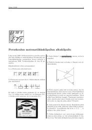
action of viscosity. The whole process (sketched in fig. 1.1) of energy transfer
from larger to smaller scale eddies is known as turbulent cascade. It is important
to remember that eddies do not correspond to real vortices, but they are just
a visual description of the triadic interactions between modes which have been
formally derived in the previous section.
Figure 1.1: Turbulent cascade à la Richardson.
Let uℓ be the rms velocity at scale ℓ and τℓ ∼ ℓ/uℓ the corresponding eddy
turnover time, i. e. the typical time for a structure of size ℓ to be significantly
15

16 1. Newtonian turbulence
deformed due to relative motion. Thus τℓ is also the typical time to transfer energy
from scales of order ℓ to smaller ones.
Dimensional analysis of the different terms in Navier-Stokes equation allows
to identify three different ranges of scales:
• injective range corresponding to large scales of order L where the forcing
pumps energy into the system;
• inertial range where both injection and viscous dissipation are negligible
so that energy simply cascades to small scales;
• dissipative range corresponding to small scales of order η where viscous
dissipation dominates and the cascade terminates.
The existence of a statistically steady state for the turbulent flow requires a
constant energy flux Π(ℓ) in the inertial range, i. e. a constant rate of energy transfer
that must be equal to the energy dissipation rate ɛ:
Π(ℓ) ∼ E(ℓ)
τℓ
∼ u3 ℓ
ℓ
= ɛ (1.46)
The above relation determines the Kolmogorov scaling of characteristic velocities
and times:
uℓ ∼ ɛ 1/3 ℓ 1/3
τℓ ∼ ɛ −1/3 ℓ 2/3
(1.47)
(1.48)
In this inertial range, the eddy turnover time at scale ℓ is much smaller than
the viscous time at the same scale τ (diss)
ℓ ∼ ℓ2 /ν; hence the energy is conserved
and transported to smaller scales.
The border between the inertial and the dissipative range is identified by the
Kolmogorov dissipative scale η, where τℓ ∼ τ (diss)
ℓ :
� � 3 1/4
ν
η ∼
(1.49)
ɛ
Below the Kolmogorov scale dissipation dominates and the velocity field is
smooth and differentiable.
1.2.2 Kolmogorov K41 theory
There is presently no fully deductive theory of turbulence explaining the basic experimental
observations of finite energy dissipation rate and power law spectrum
16

1.2. Phenomenology of turbulence 17
of exponent −5/3, in the limit of very large Reynolds number. Nevertheless, it
is possible to make assumptions compatible with these laws and leading to further
predictions. In Kolmogorov 1941 (K41) theory, hypotheses are formulated
as to reproduce the experimental behaviour of the second order structure function
(i. e. of the spectrum).
If δuℓ(x) ≡ [u(x + ℓ) − u(x)] · ℓ/|ℓ| is the longitudinal velocity increment,
then the p-th moment of its distribution:
is called longitudinal structure function of order p.
Let us reformulate Kolmogorov’s hypotheses:
Sp(ℓ) ≡ 〈(δuℓ) p 〉 (1.50)
H1 in the limit Re → ∞, all the simmetries of Navier-Stokes equation, broken
by the mechanisms producing the turbulent flow, are restored in a statistical
sense at small scales (ℓ ≪ L) and far from the boundaries;
H2 in the same limit, the turbulent flow is self-similar at small scales. A unique
scaling exponent h ∈ R therefore exists, such that:
δuλℓ(x) = λ h δuℓ(x) ∀λ ∈ R+, ∀x : |x| ≪ L (1.51)
H3 again, in the same limit, the energy dissipation rate has a finite nonvanishing
limit 0 < ɛ < ∞.
Starting from the Karman-Howarth-Monin relation [2], Kolmogorov derived
the following exact result:
four-fifths law. In the limit of infinite Reynolds number the third order (longitudinal)
structure function of homogeneous isotropic turbulence, evaluated for
increments ℓ small compared to the integral scale, is given in terms of the mean
energy dissipation rate ɛ by
S3(ℓ) ≡ 〈(δuℓ) 3 〉 = − 4
ɛℓ (1.52)
5
The four-fifths law allows to determine the value of the scaling exponent h. Under
rescaling of the increment ℓ by a factor λ, thanks to hypothesis H2, 〈(δuℓ) 3 〉 in
(1.52) is multiplied by a factor λ3h while −4 5
ɛℓ is multiplied by a factor λ, which
implies h = 1/3.
If we now consider the structure function of arbitrary order p > 0, this scales
as Sp(λℓ) = λ p/3 Sp(ℓ), so that Sp(ℓ) ∼ ℓ p/3 . Since the physical dimensions of
(ɛℓ) p/3 are those of Sp, we have
Sp(ℓ) = Cpɛ p/3 ℓ p/3
17
(1.53)

18 1. Newtonian turbulence
The dimensionless constants Cp are not known, except for the universal value
C3 = −4/5.
An interesting case corresponds to p = 2; the K41 prediction for the second
order structure function then is
S2(ℓ) ∼ ɛ 2/3 ℓ 2/3
The above scaling implies the power law energy spectrum:
E(k) = C2ɛ 2/3 k −5/3
where C2 is called Kolmogorov constant.
(1.54)
(1.55)
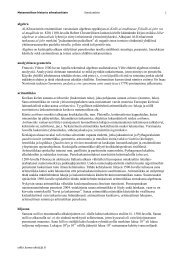
Figure 1.2: Turbulent spectra in the time domain for data from the S1 wind tunnel
ONERA [9] (Rλ = 2720, left) and a low temperature helium gas flow between
counter-rotating cylinders [10] (Rλ = 1200, right).
Longitudinal structure functions are convenient also for an experimental approach.
Indeed, longitudinal velocity increments can be obtained by means of
standard techniques such as, e. g., hot wire anemometry. Let us suppose to have
a velocity field u which can be decomposed in a mean flow U = (U, 0, 0) and
a turbulent fluctuating part u ′ = u − U whose intensity is assumed to be small
compared to the mean flow 〈|u ′ | 2 〉 1/2 ≪ U. Due to the cooling produced by the
flow, the resistance of a hot wire perpendicular to the mean flow, say parallel to
the z direction, is reduced. From the measure of this reduction, it is possible to
obtain the time series of the velocity integrated in the direction of the wire:
uN = [(u ′ x + U) 2 + u ′2
y ] 1/2 = U[1 + u′ x
U + O(u′2 x
U 2)]
(1.56)
where it has been supposed that amplitudes of fluctuations in the two directions
perpendicular to the wire are of the same order u ′ x ∼ u′ y . Within Taylor hypothesis,
18

1.2. Phenomenology of turbulence 19
i. e. assuming that for a short time delay τ the turbulent velocity field is almost
frozen and simply transported by the fast mean flow U, the time series u ′ x (t) can
be reinterpreted as a space series
u ′ x (x, t + τ) = u′ x (x − Uτ, t) (1.57)
and the structure function can be obtained.
Spectra such as (1.55) have been observed in a variety of physical situations,
from experiments in tidal channels [8], to more recent measurements in wind
tunnels [9] and in low temperature helium gas flows between counter-rotating
cylinders [10] (see fig. 1.2).
1.2.3 Intermittency
The central hypothesis of Kolmogorov K41 theory is the self-similarity of the
random velocity field at inertial range scales. Nevertheless, experimental turbulent
signals, once high-pass filtered, typically reveal intermittent features: their activity
is restricted to only a fraction of the time, which decreases with the time scale
under consideration. In other words, the velocity field can be thought as a random
alternation of quiet periods and chaotic bursts of intense fluctuations.
These intermittent features are reflected in the shape of the probability distribution
function (pdf) of velocity increments (see fig. 1.3). Experimental data
[11, 12, 13] show that the pdf is essentially gaussian at large scales (ℓ0) but, as
the scale gets smaller, it develops higher and higher tails accounting for larger and
larger probabilities of strong fluctuations. Near the Kolmogorov dissipative scale
η, the pdf takes the shape of a stretched exponential.
A convenient measure of intermittency is given by the flatness:
F(ℓ) ≡ S4(ℓ)
(S2(ℓ)) 2 = 〈(δuℓ) 4 〉
〈(δuℓ) 2 〉 2
(1.58)
Since the fourth order moment receives higher contributions from the tails of the
probability distribution function (pdf), the flatness gives a measure of the frequency
of events larger than the standard deviation. While for an intermittent
function the flatness grows with decreasing scale, either in the gaussian (F = 3)
or in the self-similar case this is not true, being F independent of the scale ℓ.
Measurements of high order structure functions [9], allowed to the detect the
intermittent nature of the turbulent velocity field, both in the dissipative and the
inertial range. The results suggest that structure functions follow power laws in
the inertial range:
Sp(ℓ) = 〈(δuℓ) p 〉 ∼ ℓ ζp (1.59)
but the exponents ζp differ from the K41 prediction ζ K41
p
19
= p/3.

20 1. Newtonian turbulence
Figure 1.3: Probability distributions, normalized with their standard deviations
σr =< δu 2 r >1/2 , of transverse velocity increments in a turbulent air jet at Rλ =
695 for different separations: r ∼ η (dotted line); r ∼ ℓ0 shifted of three decades
(long dashed line); intermediate scales (solid line) [13].
A phenomenological model of intermittency is the multifractal one, introduced
by Parisi and Frisch [14]. In the multifractal approach [14, 15], instead of global
scale invariance, local scale invariance is assumed; more specifically, hypothesis
H2 is modified into:
HMF in the limit Re → ∞, the turbulent flow possesses a range of scaling
exponents I = [hmin, hmax]. For all h ∈ I, there is a set Sh ⊂ R3 of
dimension D(h), such that for x ∈ I and ℓ → 0:
� �h δuℓ(x) ℓ
∼
(1.60)
u0
where, of course, u0 is the large scale velocity.
The structure function of order p is then expressed as a superposition, weighted
with a measure dµ(h), of different contributions originated by different scaling
exponents:
Sp(ℓ)
u p
0
�
∼
I
ℓ0
� �ph+3−D(h) ℓ
dµ(h)
ℓ0
(1.61)
where the factor (ℓ/ℓ0) 3−D(h) is the probability of being within a distance ℓ of the
set Sh. The exponent ζp can be obtained in the limit ℓ → 0 by a saddle-point
20

1.2. Phenomenology of turbulence 21
argument, which gives the relation:
ζp = inf
h [ph − D(h) + 3] (1.62)
in which one recognizes the Legendre transform of the fractal dimension D(h).
1.2.4 Acceleration statistics
The motion of test particles in a turbulent flow as they are pushed by fluctuating
accelerations is a subject of interest for a wide variety of problems, ranging from
cloud formation [16] to stirred chemical reactions and combustion processes [17].
From a more fundamental point of view, the study of acceleration statistics is
essential for transport and mixing in turbulence.
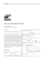
Figure 1.4: Particle trajectory in a turbulent water flow, Rλ = 970. A sphere
marks the measured position of the particle in each of 300 frames taken every
0.014ms (≈ τη/20). The shading indicates the acceleration magnitude, with the
maximum value of 12000ms −2 corresponding to approximately 30 standard deviations
[18].
A typical turbulent trajectory is shown in fig. 1.4. This is a three-dimensional
measure, with extremely high resolution in time, of the trajectory of a tracer in
a water flow [18], obtained using silicon strip detectors originally designed for
high-energy physics experiments. This trajectory shows that tracers in a turbulent
flow experience a highly irregular motion, characterized by violently fluctuating
accelerations; the particle enters the detection volume from the upper right, is
21

22 1. Newtonian turbulence
pushed to the left by a burst of acceleration and comes nearly to a stop before
being rapidly accelerated upward by a fluctuation roughly equal to 30 times the
root mean square value.
The acceleration a of a fluid particle in a turbulent flow is given by the Navier-
Stokes equation:
a ≡ du
= −∇p + ν∆u + f (1.63)
dt
Provided f is a large scale forcing and Re is large enough, the statistics of a
is essentially determined by that of pressure gradients. Experimental data [18]
indicate that the acceleration is an extremely intermittent variable and the shape
of its pdf is a stretched exponential (fig. 1.5).
Figure 1.5: Probability distribution functions of a normalized acceleration component
at three Reynolds numbers. The solid line is a stretched exponential parameterization
of the highest Rλ data, the inner dotted line is a gaussian for reference.
Inset: flatness F = 〈a 4 〉/〈a 2 〉 2 as a function of Rλ [18].
Let us now derive the shape of the acceleration pdf by means of simple phenomenological
arguments. By definition
δuτ
a ≡ lim
τ→0 τ
� δuτη
τη
(1.64)
where τη is the eddy turnover time associated with the Kolmogorov dissipative
scale η. The velocity fluctuations along a particle trajectory may be considered as
the superposition of different contributions from eddies of all sizes. In a time lag
τ the contributions from eddies smaller than a given scale ℓ are uncorrelated and
one may then write δuτ ∼ δuℓ. We assume that ℓ and τ are linked by the typical
22

1.2. Phenomenology of turbulence 23
eddy turnover time at the given spatial scale, τℓ ∼ ℓ/δuℓ. Therefore, we can write
2 (δuη)
a �
η
(1.65)
Imposing the scaling δuℓ = u0(ℓ/ℓ0) h , we have: η/ℓ0 = Re −1/(1+h) , and hence
(Rλ ∼ Re 1/2 ) we get the estimate:
a = u2 0
ℓ0
R −22h−1
1+h
λ
(1.66)
In the framework of K41 theory h = 1/3 and the only fluctuating quantity is
the large scale velocity u0. The pdf of acceleration p(a) is then simply obtained
by the change of variable p(a)da = p(u0)du0 and the assumption of gaussianity
for the statistics of the large scale velocity. This gives the stretched exponential:
p(a) ∼ a −5/9 e −a8/9
(1.67)
where the standard deviation of u0 was implicitly assumed to be unity.
From (1.66) the acceleration variance is expressed in terms of the energy dissipation
rate ɛ by:
〈a 2 〉 = u20 Rλ ∼ ν
ℓ0
−1/2 ɛ 3/2
(1.68)
known in the literature as Heisenberg-Yaglom relation. This is experimentally verified
in the limit of very large Reynolds numbers; at moderate values of Rλ there is
experimental and numerical evidence of a weak dependence of the proportionality
coefficient on ɛ.
The estimate (1.67) only roughly reproduces the large tails of experimental
acceleration probability distributions. This is not surprising, since this expression
is derived in the context of K41 theory and thus cannot take into account intermittency.
Recently, several attempts have been made to improve the agreement
between theory and experiments for Lagrangian statistics, such as acceleration.
Among these, a considerable number focuses on the construction of models based
on generalized equilibrium statistics (see, e. g., [19, 20, 21, 22], critically reviewed
in [23]).
A possible alternative approach, rooted in the phenomenology of turbulence,
is based on the multifractal model [24]. Let us briefly present its main issues. The
starting point is expression (1.66) of the acceleration, that can be rewritten as
a(h, u0) ∼ ν 2(h−1)/(1+h) u 3/(1+h)
0 ℓ −3h/(1+h)
0
(1.69)
In the multifractal framework, the scaling exponent h is allowed to fluctuate within
the interval I = [hmin, hmax]. The pdf of a can be obtained integrating (1.69) over
23

24 1. Newtonian turbulence
all h and u0, weighted with their respective probabilities, [τη(h, u0)/τℓ0(u0)] [3−D(h)]
(1−h)
and p(u0). The latter, as before, is reasonably approximated by a gaussian of standard
deviation σ2 u = 〈u20 〉. Integration over u0 gives
p(a) ∼
h∈I
�
h∈I
�
× exp
dha [h−5+D(h)]/3 ν [7−2h−2D(h)]/3 ℓ D(h)+h−3
0 σ −1
u
− a2(1+h)/3ν2(1−2h)/3ℓ2h 0
2σ2 u
�
(1.70)
From (1.70) the dependence of the acceleration moments on Rλ can be derived.
For example, in the limit of large Rλ the second order moment is given by 〈a2 〉 ∼
R χ
λ , where χ = suph{2[D(h) −4h −1]/(1+h)}. The precise value of χ depends
on the choice of D(h), but it is typically close to the K41 value χK41 = 1. In terms
of the dimensionless acceleration ã = a/σa, (1.70) becomes
�
p(ã) ∼ dhã [h−5+D(h)]/3 R y(h)
�
λ exp − 1
2 ã2(1+h)/3R z(h)
�
λ (1.71)
where y(h) = χ[h−5+D(h)]/6+2[2D(h)+2h−7]/3 and z(h) = χ(1+h)/3+
4(2h − 1)/3. Let us observe that the K41 prediction (1.67) can be recovered from
(1.71) with h = 1/3, D(h) = 3 and χ K41 = 1. Comparison with data from high
resolution DNS, as reported in [24], shows that the multifractal prediction (1.71)
captures the shape of the acceleration pdf much better than its K41 counterpart
(see fig. 1.6).
Figure 1.6: Log-linear plot of the acceleration pdf. The crosses are DNS data, the
solid line is the multifractal prediction, and the dashed line is the K41 prediction.
The DNS statistics was calculated along the trajectories of 2 × 10 6 Lagrangian
particles amounting to 1.06 × 10 10 events in total. Inset: ã 4 p(ã) for DNS data
(crosses) and the multifractal prediction [24].
24

1.3. Two-dimensional turbulence 25
1.3 Two-dimensional turbulence
Two-dimensional turbulence describes the behaviour of high-Reynolds-number
solutions of Navier-Stokes equation which depend only on two cartesian coordinates
(x, y). In this case, the third component of the velocity uz satisfies an
advection-diffusion equation without back-reaction on the horizontal (x, y) flow.
Hence, without loss of generality, one may assume that the velocity has only two
components.
There exist numerous situations, in natural flows and laboratory experiments,
which are constrained to quasi-two-dimensional motion. The most important examples
probably arise in geophysics and plasma physics. Indeed, the intermediatescale
dynamics of the oceans and the atmosphere, due to the combined effect of
their stratification and earth’s rotation, can be roughly described as being twodimensional.
Similarly, a strong magnetic field can confine the turbulent motions
of a plasma in the plane perpendicular to its axis and the dynamics can be described
by two-dimensional magneto-hydrodynamics (2D MHD) [25].
The classical theory of 2D turbulence originates from the works of of Batchelor,
Kraichnan and Leith [26, 27, 28], where it was shown that the conservation
of vorticity along streamlines, occurring in two dimensions, produces radical
changes in the behaviour of turbulence.
Finally, Navier-Stokes equation in two dimensions is less demanding on a
computational level than the three dimensional case, thus allowing to reach relatively
high Reynolds numbers in direct numerical simulations.
1.3.1 Vorticity equation
In two dimensions the incompressible velocity field u can be expressed in terms
of the stream function ψ as:
u = (∂yψ, −∂xψ) (1.72)
The vorticity field, defined as the curl of velocity ω = ∇ × u, in two dimensions
has only one nonzero component, normal to the plane of velocity, which is related
to the stream function by
ω = −∆ψ (1.73)
Instead of describing the flow in terms of the two velocity components, which
are not independent because of the incompressibility condition, it is convenient to
work with the evolution equation for the scalar field ω, obtained taking the curl of
the 2D Navier-Stokes equation. This reads:
∂ω
∂t
+ u · ∇ω = ν∆ω − αω + fω
(1.74)
25

26 1. Newtonian turbulence
The linear dissipative term on the right-hand side of (1.74) accounts for friction
between the thin layer of fluid which is considered and the rest of the three dimensional
environment. The term fω represents an external forcing that counteracts
dissipation by viscosity ν and friction α and allows to obtain a statistically steady
state.
To solve eq. (1.74) it is necessary to specify boundary conditions, which are
required to solve the Poisson equation (1.73) for the stream function. In most
studies on two-dimensional turbulence these are assumed to be of periodic type
in both the directions. The presence of realistic no-slip boundaries gives rise to a
source of vorticity fluctuations.
1.3.2 Inviscid invariants
The main difference between the two and three-dimensional problem is the conservation
of vorticity along fluid trajectories in 2D, when viscosity, friction and
forcing are ignored.
The origin of this phenomenon is due to the absence of the vortex-stretching
term (ω ·∇)u in the two-dimensional vorticity equation. In three dimensions this
term is responsible for the unbounded growth of enstrophy in the limit of infinite
Reynolds number.
In the inviscid limit ν = 0, with no forcing and friction, eq. (1.74) simply
states that the material derivative of ω vanishes:
Dω
Dt
= ∂ω
∂t
+ u · ∇ω = 0 (1.75)
thus implying conservation of vorticity of fluid particles. Moreover, all the integrals
of the form � d 2 rf(ω) are inviscid invariants of the flow. In particular, this
yields conservation of the of the enstrophy
Z = 1
�
2
d 2 r|ω| 2
If f = α = 0 in eq. (1.74), the enstrophy balance equation
(1.76)
dZ
dt = −ν〈|∇ω|2 〉 = −2νP (1.77)
states that Z is bounded since, by definition, the palinstrophy P is a positivedefinite
quantity:
P = 1
2 〈|∇ω|2 〉 = 1
�
d
2
2 r|∇ω 2 | (1.78)
26

1.3. Two-dimensional turbulence 27
Therefore, at variance with the three-dimensional case, in two-dimensional turbulence
the viscous dissipation of energy vanishes in the limit ν → 0:
dE
lim
ν→0 dt
= lim(−2νZ)
= 0 (1.79)
ν→0
but there still is dissipative anomaly for enstrophy (when friction is not considered).
The complete balance equations are:
dZ
= −2νP − 2αZ + ζ (1.80)
dt
dE
= −2νZ − 2αE + ɛ (1.81)
dt
where ɛ and ζ are, respectively, energy and enstrophy input terms. From the above
equations is clearly seen that, in the limit of vanishing viscosity, the friction term
(−2αE) is responsible for the existence of a stationary state; indeed was it α = 0
in eq. (1.81), energy would grow indefinitely. Moreover, in the same limit ν → 0,
it is known [29] that the presence of friction causes the enstropy dissipation to
vanish as well.
1.3.3 Direct and inverse cascades
Since viscous energy dissipation vanishes in the limit Re → ∞, in fully developed
two-dimensional turbulence it is not possible to have a cascade of energy with
constant flux towards small scales as in three dimensions. Indeed, the presence
of two quadratic inviscid invariants, energy and enstrophy, modifies the picture of
the turbulent cascade.
In order for both energy and enstrophy to be conserved, the net transfer by
each triad interaction must be out of the middle wavenumber into both smaller
and larger wavenumbers. Starting from the hint that interactions should act towards
producing equilibrium, a state which is never reached because of viscous
dissipation, Kraichnan showed that in two-dimensional turbulence enstrophy is
mainly transferred to small scales, where it is dissipated by viscosity, giving rise
to the direct enstrophy cascade; on the contrary, energy is transported to lower
wavenumbers, in the inverse energy cascade (see fig. 1.7).
The scaling laws in both cascades can be obtained from dimensional analysis
of Navier-Stokes equation as well as in the three dimensional case.
Inverse energy cascade
For the inverse energy cascade, the assumption of constant energy flux Π(ℓ) = −ɛ
towards large scales reproduces 3D-like scaling laws for velocities and character-
27

28 1. Newtonian turbulence
Figure 1.7: Schematic double cascading spectrum of forced (wavenumber kF )
two-dimensional turbulence.
istic times:
uℓ ∼ ɛ 1/3 ℓ 1/3
τℓ ∼ ɛ −1/3 ℓ 2/3
(1.82)
(1.83)
This means that the velocity field in the inverse cascade is rough, with scaling
exponent h = 1/3, exactly as in the three dimensional case. The prediction for
the energy spectrum is:
E(k) = Cɛ 2/3 k −5/3
(1.84)
The hypothesis of locality of interactions in the inverse cascade is consistent
with the k −5/3 spectrum. The transfer is associated with the distortion of the
velocity field by its own shear. The effective shear at a given wavenumber k
is expected to be negligibly affected by wavenumbers ≪ k because the integral
� ∞
0 k2 E(k)dk, which measures the mean square shear, converges at k = 0. Also
the contribution from high wavenumbers ≫ k is negligible because vorticity associated
with those wavenumbers fluctuates rapidly in space and time and gives a
small effective shear across distances of order k −1 .
In the absence of a large scale sink of energy, the inverse cascade can only be
quasy-steady because the peak kE of the energy spectrum keeps moving down to
ever lower wavenumbers as
kE ∼ ɛ −1/2 t −3/2
(1.85)
while the total energy grows linearly in time as E(t) = ɛt. If the energy input is
turned on for a sufficiently long time, the cascade can eventually reach the integral
28

1.3. Two-dimensional turbulence 29
scale and begins to accumulate at the lowest wavenumber. This pile-up of energy
can produce a large scale spectrum steeper than k −3 , which violates the hypothesis
of locality of interactions.
The presence of friction stops the energy cascade at the wavenumber
kE ∼ ɛ −1/2 α 3/2
(1.86)
where the energy dissipation balances the energy transfer.
In two-dimensional turbulence it is possible to demonstrate the analogous of
Kolmogorov’s four-fifths law. In the limit of infinite Reynolds number the third
order (longitudinal) structure function of two-dimensional homogeneous isotropic
turbulence, evaluated for increments ℓ small compared to the integral scale and
larger than the forcing correlation length, is given in terms of the mean energy
flux ɛ by
S3(ℓ) ≡ 〈(δuℓ) 3 〉 = 3
ɛℓ (1.87)
Together with the scaling hypothesis for the structure functions Sp(ℓ) ∼ ℓ ζp , the
three-halves law allows to obtain the equivalent of K41 theory for the inverse
energy cascade.
At variance with the three-dimensional case, where intermittency modifies the
dimensionally predicted scaling exponents, the statistics of velocity fluctuations
in the inverse-cascade range of scales is found to be roughly self-similar [30], with
small deviations from gaussianity.
Direct enstrophy cascade
At scales smaller than the forcing correlation length, the hypothesis of constant
enstrophy flux Πω(ℓ) = ζ leads to a different scaling. The enstrophy contained in
the eddies of size ℓ can be estimated as Z(ℓ) ∼ E(ℓ)/ℓ 2 ∼ u 2 ℓ /ℓ2 and its flux is
so that velocities scale as
Πω(ℓ) ∼ Z(ℓ)
τℓ
2
∼ u3 ℓ
ℓ 3
(1.88)
uℓ ∼ ζ 1/3 ℓ (1.89)
Therefore the velocity field is smooth in the direct cascade. The dimensional
prediction for characteristic times gives a single time scale τ ∼ ζ −1/3 , which
provides an estimate of the inverse of the Lyapunov exponent of the flow. The
prediction for the energy spectrum is
E(k) = C ′ ζ 2/3 k −3
(1.90)
A spectrum k −3 means that the integral � ∞
0 k2 E(k)dk, a measure of the mean
square shear, has a logarithmic divergence in the infrared cutoff. Thus the hypothesis
of locality of interactions can be violated in the direct enstrophy cascade.
29

Chapter 2
Polymer solutions
It is known since the 1940’s that the addition of small amounts of polymers to
a fluid can produce dramatic changes of its properties. Due to their molecular
structure, polymers have elastic degrees of freedom which must be taken into account
in the description of the mechanical response of the fluid to which they are
added. Indeed, while for a Newtonian fluid the stress is proportional to the deformation
rate, the coefficient being the viscosity, in an elastic material the stress
is proportional, via the Hook modulus, to the deformation itself. A solution of a
Newtonian fluid and polymers can be thought of as a mixture of these idealized
situations, because it presents features of both viscous and elastic materials, and
it is thus called a viscoelastic fluid.
The above behaviour manifests itself in a variety of spectacular phenomena.
Among these, to have an idea of the different response of Newtonian and viscoealstic
fluids, let us briefly consider the Weissenberg effect [31]. When a Newtonian
fluid is put in rotation, it is pushed away from the center by the centrifugal force
and a dip appears on the free surface, which takes the shape of a paraboloid. On
the contrary, when a rotating rod is inserted in a tank filled with a viscoelastic
fluid, the fluid tends to climb up the rod, as in fig. 2.1.
The effects produced by polymer additives in fluids range from the change
of flow stability and transition to turbulence, to the modification of mixing properties
and of transport of heat, mass and momentum. The vast bibliography by
Nadolink and Haigh [32] gives an idea of the efforts devoted to the understanding
of viscoelastic fluids’ behaviour, which is clearly of interest both from a purely
theoretical and a more application-oriented point of view.
In this chapter the basic dynamics of polymers in fluids is introduced. Starting
from a "microscopic" description in terms of single polymer dynamics, full hydrodynamic
models that are typically used to describe viscoelastic solutions will
be constructed. Finally, the phenomena of drag reduction and elastic turbulence
will be briefly introduced, as they will be discussed in further detail, or referred
31

32 2. Polymer solutions
Figure 2.1: Rod-climbing or Weissenberg effect (picture from web.mit.edu).
to, in the following chapters.
2.1 Polymer dynamics in fluids
Polymers are molecules of high molecular mass, composed by a large number of
repeating units, the monomers, joined by chemical bonds to form a long chain.
There exist both natural and synthetic polymers. Examples of the first type are
DNA, proteins, starches, cellulose, latex. Synthetic polymers are commercially
produced for a huge variety of uses; among these, we find all the materials commonly
called plastics.
In what follows, simple models describing polymer dynamics will be developed.
The essential characteristics of polymers we focus on are:
• long polymers: the degree of polymerization M, i. e. the number of monomers,
is very large, typically M ∼ 10 6 .
• flexible polymers: the angle formed by a bond connecting two monomers
is fixed. This means that at the scale of the monomer the polymer is rigid.
However, if one looks at the polymer at a scale ℓp, called persistence scale,
one sees a flexible coil. When ℓp is much smaller than the total length of the
polymer the molecule is said to be highly flexible.
• homopolymers: only a single type of monomer is present.
• no branching: we will consider only single chain molecules, though there
exist polymers formed by several branches.
32

2.1. Polymer dynamics in fluids 33
Let us now briefly state the essential characteristics that models are required
to reproduce. Because of thermal agitation, at equilibrium the molecule assumes
the aspect of a statistically spherical coil, as in fig. 2.2(a), whose average radius is
typically of the order of 0.1µm. Once elongated, polymers asymptotically relax
to the equilibrium configuration on a time scale τ. For relatively small extensions
polymers counteract elongation with a recalling force proportional to the extension
itself.
(a) (b)
Figure 2.2: (a) Sketch of the coiled equilibrium configuration of a polymer. (b) A
freely jointed chain.
2.1.1 Freely jointed chain
The simplest description of a polymer is that of the freely jointed chain [fig. 2.2(b)],
in which the molecule is approximated by a chain of M segments of length b with
random indipendent relative orientations. The different nodes of the chain are
labelled by a set of vectors Pn, with n = 1, ..., M, and the bond vectors are:
The characteristic size of the chain is :
rn = Pn − Pn−1
〈|R| 2 〉 1/2 = 〈|
M�
n=1
rn| 2 〉 1/2
(2.1)
(2.2)
which, thanks to the random independent relative orientations of the bonds, gives:
〈|R| 2 〉 1/2 = M 1/2 b (2.3)
33

34 2. Polymer solutions
Introducing the maximum extension (contour length) Rmax = Mb of the chain,
we have:
〈|R| 2 〉 = Rmaxb (2.4)
A quantity often used to characterize polymer elongation at rest is the radius
of gyration R0:
R0 ≡ 〈 1
2M2 M� M�
|Pn − Pm| 2 〉 (2.5)
n=1 m=1
which is the square mean distance between two randomly selected nodes. For
flexible polymers, it is possible to show that the following scaling holds:
R 2 0 = 〈|R|2 〉
6
= Mb2
6
(2.6)
This model is equivalent to a diffusion process: a particle moving on the segments
of the chain performs a random walk. The equilibrium pdf of the elongation
R is then obtained by the central limit theorem:
Peq(R) =
�
3
2πMb2 �3/2 3R2
−
e 2Mb2 (2.7)
The above pdf allows to determine the entropic force restoring the equilibrium
coiled configuration, once polymers have been stretched. Being Z ∝ Peq the
partition function, the free energy F reads:
F = −kBT ln Z =
3kBTR 2
2Rmaxb
+ const (2.8)
where, of course, kB is the Boltzmann constant and T the temperature. The free
energy variation due to a variation of elongation is
f = ∂F
∂R
= 3kBTR
2Rmaxb
(2.9)
meaning that the polymer as a whole behaves like a spring of elastic constant
H = 3kBT
2Rmaxb .
Direct proportionality between recalling force and extension implies a linear
relaxation ˙ R = −R/τ. A convenient estimate of the relaxation time τ has been
introduced by Zimm [33], within a different chain model:
τ � µR3 0
kBT
34
(2.10)

2.1. Polymer dynamics in fluids 35
Figure 2.3: Single DNA molecule (40µm) relaxing to the coiled state. In this
experiment a latex bead (1µm) is tethered to an end of the molecule. The DNA,
coloured with a fluorescent dye, is stretched by a uniform flow and successively
let free to relax. Images are taken at 5s time intervals, from left to right [34].
where µ is the dynamic viscosity of the solvent. Experiments with DNA molecules
[34] confirm that relaxation can be safely considered linear, provided the elongation
is small compared to the maximum extension R ≪ Rmax (see fig. 2.3).
Actually, the relaxation process can be much more complex than the simple
description of Zimm model. Several microscopic models of polymeric dynamics
have been developed to characterize this process. An introduction to this subject
can be found in the book by Doi and Edwards [35]. Nevertheless, the simple linear
relaxation is able to catch, at least qualitatively, the basic features of polymer
dynamics in fluids.
Finally, let us mention that the description of a polymer as a freely jointed
chain does not consider excluded-volume effects, which are experimentally known
to alter the scaling R0 ∼ M 1/2 of the gyration radius with the degree of polymerization.
The scaling exponent is, indeed, found to be ν = (0.55 ÷0.6). The origin
of these effects is the possibility that segments of the chain have, in the model, to
intersect or superpose to each other, which is not realistic. A better approximation
of the chain dynamics is based on a self-avoiding random walk. While the theory
of the standard random walk is quite simple, the treatment of the self-avoiding
problem is more difficult. A theoretical estimation of ν has been given by Flory
[36] for spatial dimensionality d < 4:
ν = 3
d + 2
(2.11)
which, for d = 3, gives the value ν = 3/5 = 0.6, not far from the experimental
measures; in two dimensions, Flory’s result is exact. When d ≥ 4 the value
ν = 1/2 of the ideal chain is recovered, meaning that the segments have "enough
room" to avoid each other.
35

36 2. Polymer solutions
2.1.2 Weissenberg number
The behaviour of polymers in a flow critically depends on the gradients of the
velocity field. In a non-homogeneous flow, the polymer molecule can be deformed
into an elongated shape and its extension R can be significantly larger than the
equilibrium value R0. The deformation is determined by the competition between
the stretching exerted by velocity gradients and the relaxation due to Brownian
collisions with molecules of the fluid.
The relative strength of stretching with respect to relaxation is quantified by
the adimensional Weissenberg number:
Wi ≡ γτ (2.12)
defined as the product of the characteristic velocity gradient γ and the relaxation
time τ. When Wi ≪ 1 relaxation is fast and polymers stay in their coiled configuration.
For Wi ≫ 1, on the contrary, polymers are substantially elongated. The
transition point is called coil-stretch transition and corresponds to Wi = O(1).
The coil-stretch transition has been demonstrated to occur under general conditions
in unsteady flow [37, 38]; in the case of steady flow, it is present in purely
elongational flows, while it can be suppressed by rotation, becasue polymers do
not always point in the stretching direction [39].
In a turbulent velocity field polymers are stretched by a chaotic smooth flow,
because their linear size is typically smaller than the Kolmogorov dissipative scale
η. In such a case, the characteristic velocity gradient is measured by the Lagrangian
Lyapunov exponent λ, that is the average logarithmic divergence rate of
initially very close trajectories, and the Weissenberg number is:
Wi = λτ (2.13)
The Lyapunov exponent λ of a turbulent flow is, by dimensional analysis, the
inverse of the shortest eddy turnover time. Within K41 scaling, this is τη ∼
ɛ −1/2 ν 1/2 , so that λ ∼ Re 1/2 , as well as Wi ∼ Re 1/2 ; hence at a critical Reynolds
number, the coil-stretch transition occurs.
The growth of the molecule size R is limited by the back reaction of polymers
themselves on the flow. When these are significantly elongated, elastic stresses
become comparable to the visocus ones and, consequently, the flow can be modified.
Specifically, this mechanism can reduce the Lyapunov exponent [39, 40],
i. e. stretching, giving rise to a dynamical steady state characterized by a constant
average elongation. For the sake of clearness, in the following, the Weissenberg
number will always be defined in terms of the Lyapunov exponent of the Newtonian
fluid flow: Wi ≡ λNτ.
36

2.1. Polymer dynamics in fluids 37
2.1.3 Dumbbell model
A model which is very often used for its simplicity is the dumbbell model [41],
where the complex structure of the polymer molecule is replaced by a couple of
beads of negligible mass, connected by a spring. Such a spring has the same
properties of an entire freely jointed chain (see sec. 2.1.1) of Hook modulus
H = 3kBT
2Rmaxb . The evolution of the dumbbell end-to-end vector R = x2 − x1
is determined by different contributions: the hydrodynamic drag force acting on
the polymer, thermal noise, and the elastic recalling force of the spring. In a homogeneous
flow, the equation of motion for R then is:
˙R = − H
R + Bξ (2.14)
β
where β is the friction coefficient and ξ is a zero mean Brownian process with
correlation 〈ξi(t)ξj(t ′ )〉 = δijδ(t − t ′ ). The relaxation time is clearly introduced
as:
τ ≡ β
H
(2.15)
The dependence of the constant B on the gyration radius R0 and the relaxation
time τ can be derived as follows. The formal solution of eq. (2.14) allows to
estimate the long time behaviour of the square mean elongation as 〈R2 〉 ∼ τB2
. At 2
is comparable
equilibrium, the elastic energy of the spring U ∼ H〈R2 〉eq ∼ HR2 0
to the thermal energy kBT , which implies B = (2R2 0 /τ)1/2 .
U ( x1)
R(t)
U (x2 )
Figure 2.4: Sketch of the dumbbell in a velocity field u(x).
In a non-homogeneous flow, polymers can also get stretched, because of different
velocities of the two beads (see fig. 2.4). Therefore, a term ˙ R = u(x2, t) −
u(x1, t) must be added to the evolution equation (2.14). Since the flow is smooth
at the scale of the polymer, we can approximate this stretching term with the ve-
37

38 2. Polymer solutions
locity gradient, and finally write the complete equation of motion:
˙R = (R · ∇)u − 1
R +
τ
�
2 2R0 ξ (2.16)
τ
The linear description of the dumbbell model is adequate for relatively small
elongations R ≪ Rmax. When this condition is not anymore fulfilled, it is reasonable
to expect that different structures will have different elasticities, namely for
very large elongations the friction coefficient β depends on the elongation itself,
and so does the relaxation time. A possible generalization taking into account
these effects is the Finitely Extensible Nonlinear Elastic model (FENE) [31], in
which τ → τ R2 max −R2
R 2 max−R 2 0
. This simple modelling works particularly well for syn-
thetic polymers (such as PolyEthileneOxide and PolyAcrylaMide).
Estimating the friction coefficient as β = 6πµR0 and plugging this expression
in (2.15), the Zimm relaxation time (2.10) is found. This unique characteristic
time has to be intended as the slowest relaxation time of the polymer dynamics.
In other words, the dumbbell model retains only the fundamental elastic mode
of the polymer chain. Although higher oscillatory modes, with faster relaxation
times, have been experimentally observed in DNA [42], they can be only weakly
excited by the velocity gradients of a turbulent flow. Consequently, in a simplified
rheological model it is enough to keep only the slowest relaxation mode.
Coil-stretch transition
The dumbbell model is able to reproduce the coil-stretch transition, happening
when the stretching operated by the flow overcomes the relaxation of polymers. In
what follows the main points of the theory developed in ref. [38] will be presented.
Since our interest is now focused on the competition between stretching by
velocity gradients and relaxation, thermal noise is irrelevant and the evolution
equation (2.16) for the end-to-end separation vector R of the dumbbell, for the
component Rα, reads:
d
(2.17)
dt Rα = Rβ∂βuα − Rα
τ
To get rid of inessential degrees of freedom responsible for the orientation of
the molecule, we can write R = Rn, passing to the modulus R of the vector R.
Then we obtain from eq. (2.17):
dρ
dt
1
= ζ −
τ
(2.18)
dnα
dt = nβ∂βuα − ζnα (2.19)
R = R0e ρ , ζ = nαnβ∂βuα (2.20)
38

2.1. Polymer dynamics in fluids 39
For turbulent flows, where the velocity field u is a random function of time,
a statistical approach is needed. Specifically the problem can be attacked with a
large deviations approach. Integration of eqs. (2.18)-(2.19) brings:
ρ(t) = ρ0 + z − t
, z =
τ
� t
dt
0
′ ζ(t ′ ) (2.21)
where ρ0 is the value of ρ at t = 0. The integral z in eq. (2.21) has universal properties,
for times much larger than the correlation time τζ of the random process ζ,
which in a turbulent flow is estimated as the characteristic time of the Lagrangian
motion on the vicous scale. For t ≫ τζ, the variable z is the sum of a large number
of independent variables and the statistics of fluctuations of z near its mean value
can be deduced by the central limit theorem. In order to study large deviations, a
more general formulation is needed, corresponding to the following pdf of z:
G(t, z) ≈
�
λ = 〈ζ〉, ∆ =
1
z−λt
√ e
−tS( t ) (2.22)
2π∆t
dt ′ � 〈ζ(t)ζ(t ′ )〉 − λ 2�
(2.23)
where the "entropy density" S is a positive convex function and λ is the principal
Lyapunov exponent of the flow.
In order to derive the probability distribution of molecular elongations, let us
consider typical fluctuations determining the largest contribution to the pdf itself.
If the polymer initially has a nearly equilibrium shape (ρ0 ∼ 1) and it is successively
stretched by velocity gradients up to ρ ≫ 1, then the function G(t, ρ+t/τ)
provides an estimate of the contribution due to fluctuations of stretching period t.
This has a sharp maximum at t∗ = ρ/β, determined from dG(t, ρ + t/τ)/dt = 0,
where β is such that
βS ′ (β + 1
τ
− λ) − S(β + 1
τ
− λ) = 0 (2.24)
The probability distribution is thus dominated by fluctuations of duration t∗, which
means:
(2.25)
or, equivalently, in terms of R:
1
−t∗S(β+
G ∼ G(t∗, ρ + t∗/τ) ∼ e τ −λ)
P(R) ∼ R α 0R −1−α
α = S ′ (β + 1
τ
(2.26)
− λ) (2.27)
Let us observe that the characteristic value of the velocity gradient for relevant
fluctuations is given by ζ ∼ ρ/t∗ + 1/τ and is of order 1/τ.
39

40 2. Polymer solutions
The convexity and positivity of the function S ensure that α is positive if λ <
1/τ. As it is clear from eq. (2.27), α decreases with increasing λ, tending to zero
when λ approaches 1/τ. In the latter case, the quadratic approximation S(x) ≈
x 2 /(2∆) holds, leading to:
β = 1
− λ (2.28)
τ
α = 2
� �
1
− λ
(2.29)
∆ τ
The above discussion can be interpreted as the criterion for the coil-stretch transition.
When the value of the Weissenberg number Wi = λτ is smaller than
unity, i. e. for α > 0, the normalization integral � dRP(R) is determined by small
R and the majority of polymers have nearly equilibrium size. Above unity, instead,
α < 0 and the normalization integral diverges at large R; then most of the
molecules are strongly stretched.
40

2.2. Hydrodynamic models 41
2.2 Hydrodynamic models
The previous microscopic models describe the behaviour of a single polymer in
a fluid, but they do not include the back-reaction that polymers have on the flow.
In order to take into account this feedback mechanism it is necessary to move
to a macroscopic hydrodynamic description. Indeed, the elastic properties of the
solution require to include an extra stress term in the law of momentum conservation.
This elastic stress term provides the macroscopic description of polymer
back-reaction on the flow.
2.2.1 Oldroyd-B model
A simple linear viscoelastic model is the widely used Oldroyd-B model [31],
based on the dumbbell model.
The passage from the microscopic to the macroscopic point of view requires to get
rid of microscopic degrees of freedom, such as thermal noise. Polymer behaviour
is conveniently described by the conformation tensor:
σij ≡ 〈RiRj〉
R 2 0
(2.30)
where the average is taken over thermal noise or, equivalently, over a small volume
containing a large number of molecules. By construction the tensor σ is
symmetric, positive definite and its trace trσ is a measure of the square polymer
elongation. The evolution equation for the conformation tensor follows from the
linear equation (2.16) and reads:
∂tσ + (u · ∇)σ = (∇u) T · σ + σ · (∇u) − 2
(σ − 1) (2.31)
τ
where τ is the polymer relaxation time defined in eq.(2.10) and the matrix of velocity
gradients is defined as (∇u)ij = ∂iuj. The conformation tensor is normalized
with the equilibrium size R0 and therefore in absence of fluid flow it relaxes
to the unit tensor 1.
Equation (2.31) must be supplemented by the evolution equation for the velocity
field, which is derived from the momentum conservation law:
Dui
Dt = fi + 1 ∂Tij
ρ ∂xj
(2.32)
where f is the sum of body forces per unit mass and T is the stress tensor of the
fluid.
41

42 2. Polymer solutions
The stress tensor of a Newtonian fluid is linear in the deformation rate tensor
eij = 1/2(∂jui + ∂iuj) and, in the incompressible case, is expressed by [6]:
T N ij = −Pδij + µ(∂jui + ∂iuj) (2.33)
where µ is the dynamic viscosity and P pressure.
In the case of a viscoelastic solution, the stress tensor is given by the sum of
the Newtonian stress tensor T N and the elastic stress tensor T P , which takes into
account elastic forces due to the presence of polymers. While for a Newtonian
fluid the stress tensor is proportional to the deformation rate tensor via the viscosity,
in the Hookean approximation for the elasticity of the single polymer, the
elastic stress tensor is proportional via the Hook modulus to the deformation tensor
Tij = nHRiRj. The elastic stress tensor per unit volume of fluid is obtained
summing the average contribution given by each polymer:
T P ij = nH〈RiRj〉 = nHR 2 0 σij
(2.34)
where n is the concentration of polymer molecules.
For an incompressible fluid of constant density ρ, plugging the expression of
the stress T = T N + T P in the momentum conservation law, one obtains:
∂tu + (u · ∇)u = −∇P + ν∆u + 2νη
∇ · σ + f (2.35)
τ
The solvent kinematic viscosity is denoted by ν = µ/ρ and here η is the zero-shear
contribution of polymers to the total viscosity of the solution νT = ν(1 + η):
η = nHR2 0 τ
2µ
(2.36)
Equation (2.35) is a generalization of Navier-Stokes equation for the viscoelatic
solution and together with eq. (2.31) completely determines the dynamics
of Oldroyd-B model.
Viscosity renormalization
In the limit τ → 0, the elastic force originated from thermal motion keeps the
molecules near their equilibrium configuration, and the polymer solution is expected
to behave like a Newtonian fluid. Indeed, a perturbative expansion in τ for
the conformation tensor
σij = σ (0)
ij
substituted in eq. (2.31) gives at zero and first order:
σ 0 ij = δij; σ (1)
ij
+ τσ(1)
ij + O(τ2 ) (2.37)
= 1
2 (∂jui + ∂iuj) = eij
42
(2.38)

2.2. Hydrodynamic models 43
Therefore, at first order in τ the elastic stress is proportional to the deformation
tensor
T P ij = nHR 2 0[δij + τeij + O(τ 2 )] (2.39)
and the fluid is Newtonian up to higher order corrections O(τ 2 ). Nevertheless, the
presence of polymers affects fluid properties also in this Newtonian limit, because
the fluid is partially trapped in the coiled polymers, producing a change of the
total viscosity of the solution µT , which is renormalized as:
Energy balance
µT = µ + 1
2 nHR2 0τ = µ(1 + η) (2.40)
The free energy of the viscoelastic fluid is the sum of kinetic and elastic contributions:
�
F = d 3 �
1
x
2 ρu2 + ηνρ
�
[trσ − log det σ]
τ
(2.41)
where the last term represents the entropy of polymer molecules. In order to
compute the free energy time derivative, let us separately consider the rate of
change of different contributions. Through eqs. (2.31)-(2.35) one obtains:
u 2
2 = f · u − ν(∂iuj) 2 − ην
τ [σij∂jui + σij∂iuj] (2.42)
d
dt
d
dt trσ = [σij∂jui + σij∂iuj] − 2
tr[σ − 1] (2.43)
τ
d
2
log det σ =
dt τ tr[σ−1 − 1] (2.44)
The forcing pumps kinetic energy into the system, that is partially dissipated by
viscosity and polymer relaxation. The term σij∂jui+σij∂iuj, representing the exchange
between kinetic and elastic energy, does not have a definite sign. Summing
together the different contributions, the free energy rate of change is:
�
∂F
= ρ d
∂t 3 �
x f · u − ν(∂iuj) 2 − 2ην
τ2 tr[σ − 21 + σ−1 �
] (2.45)
Since the conformation tensor is positive definite and symmetric, it can be
decomposed as the product of two symmetric matrices S:
σij = SikSkj
(2.46)
Using this decomposition, the trace term in eq. (2.45), representing the energy
dissipation rate due to polymers, can be rewritten as
tr[σ − 21 + σ −1 ] = tr[(S − S −1 ) 2 ] (2.47)
43

44 2. Polymer solutions
which shows that it has a definite sign.
In a statistically steady state the average free energy is constant and the energy
balance reads:
ɛI = ν〈(∂iuj) 2 〉 + 2ην
τ2 � � −1
〈trσ〉 − 2tr1 + 〈trσ 〉 (2.48)
where ɛI is the average energy input per unit mass. Assuming kinetic energy and
polymer elongation are statistically constant, it follows that the average entropy
production rate vanishes:
〈trσ −1 〉 − tr1 = 0 (2.49)
and the entropy of polymer molecules is conserved.
2.2.2 FENE-P model
The linear Oldroyd-B model is based on the assumption that polymers can be
modeled as Hookean springs and, consequently, it allows infinite extension of
polymer molecules. This is clearly unphysical because the polymer end-to-end
separation R is bounded by the maximum length Rmax. When R approaches
Rmax, elastic nonlinearities become important and the linear approximation fails.
A more refined, but still conceptually simple, description is that of FENE-P model
[31], where the elastic constant H is replaced by the function:
H(R) = H R2 max − R2 0
R2 (2.50)
max − R2
diverging for R → Rmax, which means that the recoil force becomes infinite when
the polymer is extremely stretched.
However, the introduction of nonlinearities produces a non-closed evolution
equation for the conformation tensor 〈RiRj〉. A commonly accepted closure is
the Peterlin approximation [43], consisting in a pre-averaging in the nonlinear
function:
H(R 2 ) → H(〈R 2 〉) = H R2 max − R2 0
R2 max − 〈R2 〉
(2.51)
The coupled equations for the conformation tensor and the velocity field, in
the FENE-P model are:
∂tu + (u · ∇)u = −∇P + ν∆u + 2ην
H(trσ)∇ · σ + f (2.52)
τ
∂tσ + (u · ∇)σ = (∇u) T · σ + σ · (∇u) − 2
(H(trσ)σ − 1) (2.53)
τ
where the nonlinear factor has been rewritten as:
H(trσ) = trmax − tr1
(2.54)
trmax − trσ
44

2.2. Hydrodynamic models 45
with trmax = R 2 max /R2 0 .
The FENE-P model is able to reproduce features of polymer solutions not captured
by Oldroyd-B model, like the shear thinning, i. e. the decrease of viscosity
at increasing shear rates. Moreover, the finite molecular extensibility reduces the
onset of numerical instabilities due to strong gradients of the conformation tensor
field. For these reasons this model is generally adopted in numerical simulations
of viscoelastic channel flows [44].
45

46 2. Polymer solutions
2.3 Drag reduction
Since the work of the chemist Toms [45], it is known that the addition of small
amounts of polymers to a turbulent flow drastically reduces the friction drag.
Specifically, Toms observed that the addition of a few parts per million in weight
of long chain polymers to a pipe flow has the consequence of reducing the drag of
about 80%.
Friction drag in a pipe flow is usually quantified by the adimensional Fanning
friction factor f:
f = ∆P
ρU2 R
L
(2.55)
where R is the radius of the pipe, ρ is the fluid density, ∆P is the pressure drop on
a distance L and U is the mean velocity across the section. Physically, the friction
factor is the ratio of the external pressure difference sustaining the motion, and the
kinetic energy of the fluid. A significant reduction of this factor thus allows to let
a fluid flow in a pipe at a much lower cost in terms of energy, which clearly has a
high relevance for practical applications.
Figure 2.5: A schematic illustrating the onset of drag reduction and the MDR
asymptote in Prandtl-Karman coordinates. The Prandtl-Karman law corresponds
to the turbulent behaviour of Newtonian fluids. The dotted line qualitatively represents
the friction reduction in the viscoelastic case. The dashed line is for a larger
polymer concentration.
In Newtonian flows the drag coefficient f is a function of the Reynolds number,
which is Re = 2RU/ν for a pipe flow. The dependence is conventionally
shown in Prandtl-Karman (P-K) coordinates: 1/ √ f versus log(Re √ f) (see
46

2.3. Drag reduction 47
fig. 2.5). In the laminar regime the drag decreases as Re −1 until a critical Reynolds
number is reached. Transition to turbulence causes a sudden increase of the coefficient
f which, in fully developed turbulence, almost reaches a constant value
with only a weak logarithmic dependence on Re, corresponding to a straight line
in P-K coordinates.
Dilute polymer solutions deviate from the Prandtl-Karman law: below a critical
value of Re their behaviour is similar to that of a Newtonian fluid, but at larger
Reynolds numbers the drag is drastically reduced with respect to the Newtonian
case and it finally reaches a universal asymptote, independent of the specific type
of polymer and of the concentration, known in the literature as Maximum Drag
Reduction asymptote (MDR).
Many theories have been proposed to explain what is the basic physical mechanism
of the drag reduction phenomenon. Lumley [46] proposed a quantitative
approach based on the phenomenology of the channel flow. Another approach is
due to de Gennes [47], who suggested an elasticity-based criterion. Much effort
to the understanding of the problem has been dedicated also by Piva, Casciola and
coworkers [44], by Procaccia and coworkers [48], by Benzi and coworkers [49].
Finally, recent experimental results are reported in [50, 51, 52]. Despite the considerable
number of studies, a quantitative fully satisfactory explanation of drag
reduction is still lacking, and the phenomenological theories are not universally
accepted [51]. The experimental and theoretical studies on drag reduction have
been performed in wall bounded flows, due to technological and industrial applications.
It is worth remarking that this effect can take place also in the absence of
material boundaries [53].
47

48 2. Polymer solutions
2.4 Elastic turbulence
A remarkable phenomenon of recent experimental discovery [54, 55, 56, 57] is the
onset of elastic turbulence. This effect appears in a somehow opposite limit in the
space of stability parameters of the flow, with respect to drag reduction. Whereas
drag reduction is a high Reynolds number phenomenon, elastic turbulence occurs
in the limit of vanishing Re, provided the elasticity El ≡ Wi/Re is high enough.
The presence of polymers modifies the stability of a laminar flow. Indeed,
when stretched by a primary shear flow, polymers can trigger elastic instabilities.
These instabilities give rise to a secondary flow that further stretches the
molecules until a stationary state is reached. Such a state displays features typical
of turbulent flows, such as spatial and temporal irregular behaviour, with a broad
range of active scales (see fig. 2.6). The possibility to achieve turbulent states for
arbitrarily small Reynolds numbers is clearly very important for mixing related
applications in microchannel flows [56, 58], where mixing efficiency is limited by
the practical difficulty of reaching large Re.
Figure 2.6: Representative snapshots of elastic turbulence in a flow generated by
two coaxial rotating disks. [(a), (b)] Polymer solution at Wi = 6.5, Re = 0.35;
[(c), (d), (e)] polymer solution at Wi = 13, Re = 0.7; (f) pure solvent at Re = 1
[57].
A measure of elastic turbulence, as suggested in [55], is ratio between the
average shear stress and its corresponding value for a laminar flow. The results
48

2.4. Elastic turbulence 49
reported refer to a flow between two coaxial rotating disks. When the relative
angular velocity of the plates was increased the rescaled shear stress significantly
growed, exhibiting a sharp transition. The maximum stress value was found to
correspond to that of a Newtonian flow at Re ∼ 10 4 , whereas the measures were
taken at Re < 1, showing the elastic origin of this effect.
Numerical analysis of elastic turbulence in a two-dimensional flow will be the
subject of chapter 5.
49

Chapter 3
Phase separation in binary fluids
The quenching of a system from a disordered phase into an ordered one produces
a time dependent growth process of ordered regions. The temporal evolution of
these regions is the subject of phase ordering dynamics, in which the problem is
approached by means of a statistical description based on rather general forms of
equations of motion for an order parameter [59, 60]. The generality of the approach
and the universality properties of the coarsening process make the subject
of interest for a varied number of physical systems ranging from solid alloys, to
polymer blends, multiphase fluids and nematic liquid crystals [60, 61, 62, 63].
The first to address the problem were, in the late 1950’s, Cahn and Hilliard [64]
who investigated the behaviour of metallurgical systems, specifically the spinodal
decomposition of binary alloys. Similar phenomena occur in the phase separation
of binary fluids, i. e. fluids composed by either two phases of the same chemical
species, or phases of different composition. In this case, however, the phenomenology
is complicated by the interplay with the fluid dynamics. For instance,
since Siggia’s seminal work [61] it is well known that hydrodynamics may accelerate
the domain growth (see references [65] and [66] for recent developments in
three- and two-dimensional fluids, respectively). Finally, by assuming more complex
algebraic structures for the order parameter, such as vector and tensor fields
rather than the scalars usually considered, it is possible to describe phase ordering
in nematic liquid crystals [60].
This chapter is intended as an introduction to the physics of phase separation
in binary fluids, in view of a study on the interaction between turbulence and
domain growth, presented in chapter 6. The main thermodynamical aspects are
introduced and growth laws are discussed, both in the case of a fluid at rest and in
presence of a hydrodynamic velocity field.
51

52 3. Phase separation in binary fluids
3.1 Thermodynamics of binary mixtures
Let us consider the cooling of a fluid consisting of two species A and B, starting
from a completely mixed state. Below a critical temperature Tc , the originally
homogeneous phase separates into distinct A-rich and B-rich components and the
system spontaneously evolves into two phases separated by an interface.
The thermodynamic behaviour of the system can be understood by considering
the free energy F. Assuming the volume is fixed, this is a functional of a single
composition variable, accounting for the local fraction of the two fluids:
θ(x, t) ≡ nA − nB
nA + nB
(3.1)
where nA,B(x, t) are the number densities of fluid A and B, respectively, having
assumed unit mass for A and B particles.
In what follows, we will focus the attention on phase separation taking place
through spinodal decomposition [60, 61, 62, 65].
3.1.1 Spinodal decomposition
When a binary fluid is quenched into the coexistence region of its phase diagram
(see fig. 3.1) it can phase separate in two different ways. The first mechanism
occurs when the point to which the fluid is quenched is near the binodal. In this
case phase separation generally proceeds via nucleation of droplets of one phase
forming in the other phase. For example, if the fluid is quenched to a state point
inside the binodal on the liquid side, then bubbles of the gas phase can nucleate in
the bulk of the metastable liquid.
However, if the fluid is quenched to a state point well inside the binodal, then
a different separation mechanism, called spinodal decomposition, prevails. This
type of decomposition is characterized by the formation of a bicontinuous structure
of the two phases. Indeed, below the spinodal line the free energy changes
curvature and the system becomes locally unstable. The free energy can then be
lowered, in any local neighbourhood, by creating two domains whose composition
differs only infinitesimally from the initial one. Accordingly, infinitesimal
fluctuations will grow by diffusion until there is local coexistence of domains at
compositions approaching the equilibrium values of the single phases.
In order to describe this process, it is convenient to set up a continuous formulation
in terms of the coarse-grained order parameter field θ(x, t). The Landau-
Ginzburg free energy of the mixture is:
� � 2 ξ
F[θ]= dx
2 |∇θ|2 �
+ V (θ)
(3.2)
52

3.1. Thermodynamics of binary mixtures 53
Figure 3.1: Phase diagram for spinodal decomposition. Below the critical temperature
Tc the system starts to separate, whereas for higher temperatures it remains
completely mixed.
where V (θ) is a standard double well potential (fig. 3.2):
V (θ) = 1
2 r(T)θ2 + 1
4 uθ4
(3.3)
The coefficient r(T) ∝ (T − Tc) in (3.3) becomes negative at low temperatures
T < Tc, and the resulting two minima of V correspond to the equilibrium values
θ = ±1 in the bulk phases. Since the interest is here on quenches into the ordered
phase, it is reasonable to assume T = 0 and |r| = |u| = 1; moreover, we adopt
the convention V (0) = 0, so that V (±1) = −1/4. The gradient term penalizes
the formation of sharp gradients in composition and ξ gives the length scale of the
interface width.
3.1.2 Surface tension
The gradient term in the free energy functional (3.2) provides a nonzero surface
tension. This can be calculated as follows [60, 65]. Stationarity of F requires
ξ 2 ∆θ = V ′ (θ) (3.4)
Let us consider a flat interface; introducing a coordinate g normal to it and setting
θ(0) = 0, integration of eq. (3.4) across the domain wall gives
ξ 2
2
� �2 dθ
= V (θ) − V (±1) (3.5)
dg
53

54 3. Phase separation in binary fluids
0.3
0.2
0.1
2 �1 1 2 Θ
�0.1
�0.2
V�Θ�
Figure 3.2: Model potential for phase separation.
Surface tension is the energy per unit area of the wall:
�
σ ≡ dg ξ 2 |∇θ| 2
interface
Using (3.5) and the fact that ∇θ = 0 in the bulk, the above expression becomes
σ =
� +1
dθ ξ 2
−1
1/2 [V (θ) − V (±1)] 1/2
(3.6)
(3.7)
Given a form of the potential V (θ) the value of surface tension can thus be calculated.
Let us observe that the order parameter varies smoothly in the interface
region and saturates to θ = ±1 in the bulk of the domains. Then, it follows that σ
is localized in the domain wall, and that the driving force for the domain growth is
the wall curvature, since the energy of the system can decrease only by reducing
the total wall area.
3.2 Coarsening in a fluid at rest
In phase separation the order parameter is conserved on average, due to the local
exchange of particles of species A and B, which leads to a diffusive evolution
equation, known as Cahn-Hilliard equation. In absence of any external flow, this
reads:
∂θ
∂t
= Γ∆
� �
δF
= Γ∆µ (3.8)
δθ
where Γ is a mobility parameter that, here and in the following, will be assumed
constant, and µ = −θ+θ 3 +ξ 2 ∆θ is the chemical potential governing the exchange
54

3.2. Coarsening in a fluid at rest 55
of particles. It is worth remarking that Cahn-Hilliard equation can be written in
the form of a continuity equation:
∂tθ = −∇ · j (3.9)
j = −∇µ (3.10)
where adimensional units have been introduced by rescaling of lengths with ξ and
of times with the diffusive time tm = ξ 2 /Γ.
3.2.1 Domain growth
After the temperature quench phase separation starts, forming, in a short time of
the order of tm, well defined domains of the single phases, which then grow until
complete separation is achieved.
Figure 3.3: DNS of Cahn-Hilliard equation at resolution 512 2 . Snapshots of the
composition field θ at times growing from left to right. Black/white codes θ ± 1.
Inspection of a time sequence, as the one shown in fig. 3.3, suggests that domain
growth is a scaling phenomenon, provided that the typical domain size L(t)
is larger than the interface width and smaller than the whole system size. In this
range, the growth law can be derived according to the following argument [60].
In the bulk of a single phase the order parameter is constant, so that ∂tθ = 0
and the chemical potential obeys the Laplace equation
∆µ = 0 (3.11)
From the behaviour at the boundaries, it can be inferred that
µ ∼ σ
L
(3.12)
where σ is surface tension and 1/L is the curvature of the domain wall. The
interface velocity is v ∼ j ∼ ∇µ. Estimating the gradient as 1/L, the equation of
motion for L then is:
dL
dt
= σ
L 2
55
(3.13)

56 3. Phase separation in binary fluids
Integration of eq. (3.13) gives the scaling L(t) ∼ (σt) 1/3 ; reinserting the physical
dimensions, we finally get:
�
t
L(t) ∼ ξ
tm
� 1/3
3.3 Hydrodynamics and coarsening
(3.14)
A detailed description of phase separation in fluids requires to consider hydrodynamic
effects [60, 62, 65]. To do this Cahn-Hilliard equation must be modified
to include an advective term, accounting for transport of the order parameter operated
by a fluid flow. Moreover, coupling with Navier-Stokes equation for the
velocity field must be considered.
The interaction between coarsening and fluid dynamics arises as a consequence
of inhomogeneities in composition. These are controlled by the chemical
potential µ = δF/δθ, which describes the variation of free energy resulting from
a small local change in composition. If the latter is not uniform, then a thermodynamic
force density −θ∇µ acts on the fluid. The two species are pulled in
opposite dircetions by the chemical potential gradient and the net force vanishes
only if there is a single fluid or when the two fluids are perfectly mixed, i. e. when
θ = 0. The evolution equations then become:
∂tθ + v · ∇θ = Γ∆µ = Γ(−∆θ + ∆θ 3 − ξ 2 ∆ 2 θ) (3.15)
ρ[∂tv + (v · ∇)v] = −∇p + µv∆v − θ∇µ + f (3.16)
where ρ = nA + nB is the mean fluid density, v is the (incompressible) velocity
field, p the pressure, µv dynamic viscosity and f an external stirring source.
From eq. (3.16) it is seen that the order parameter is now an active field, since
it is not simply transported by the flow, but it is able to react on it. Let us now
rewrite the feedback term in a different manner:
−θ∇µ = −ξ 2 ∆θ∇θ + ∇
�
1
2 θ2 − 3
4 θ4 + ξ 2 �
θ∆θ
(3.17)
Now, the last term on the right-hand side of eq. (3.17) can be reabsorbed in the
pressure gradient, and the stress tensor results modified by this chemical pressure
term, with respect to the Newtonian case.
Finally, the equations of motion are:
∂tθ + v · ∇θ = Γ∆µ = Γ(−∆θ + ∆θ 3 − ξ 2 ∆ 2 θ) (3.18)
∂tv + (v · ∇)v = −∇p + ν∆v − ξ 2 ∆θ∇θ + f (3.19)
56

3.3. Hydrodynamics and coarsening 57
where ν = µv/ρ is kinematic viscosity and it has been assumed ρ = 1.
Observe that eq. (3.19) formally is the MHD equation for the velocity field,
provided one identifies the composition variable with the magnetic vector potential.
A discussion on the similiraties in the phenomenology of MHD and that of
phase separation can be found in ref. [62].
3.3.1 Growth laws
When hydrodynamics is taken into account, the coupling between Cahn-Hilliard
and Navier-Stokes equations strongly limits the possibility to derive growth laws
for the typical domain size. Nevertheless, some dimensional arguments can help
finding out how fast domains grow in different regimes individuated by the relative
strength of interfacial contributions with respect to the hydrodynamic ones.
Let us now reconsider eqs. (3.18)-(3.19) in absence of external forcing, i. e. for
f = 0. Then, the only driving force for the velocity field is the feedback term
−ξ 2 ∆θ∇θ. In order to compare different contributions, we rescale time, length
and velocity by means of natural units that can be defined in terms of the coarsening
parameters ξ and Γ, namely:
t → t
tm
; tm = ξ2
Γ
(3.20)
x → x
; lm = ξ (3.21)
lm
v → v
vm
; vm = Γ
ξ
After rescaling, the evolution equations become:
(3.22)
∂tθ + v · ∇θ = −∆θ + ∆θ 3 − ξ 2 ∆ 2 θ (3.23)
∂tv + (v · ∇)v = ν λξ2
∆v − ∆θ∇θ (3.24)
Γ Γ2 where λ = 1 is put only for dimensional reasons, its dimensions being those of a
squared velocity. Let us discuss different regimes, assuming the initial condition
v = 0 for eq. (3.24).
• If Γ is extremely high, such that λξ 2 /Γ 2 ≪ 1, the velocity remains very
small and eq. (3.24) is almost not effective, allowing to disregard the advective
term in eq. (3.23). The system then evolves according to Cahn-Hilliard
equation and the domain size grows as L(t) ∼ t 1/3 .
• If ν/Γ ≫ λξ 2 /Γ 2 , then viscous damping overcomes the forcing produced
by composition inhomogeneities and, therefore, we fall again in the previous
case, and hence L(t) ∼ t 1/3 .
57

58 3. Phase separation in binary fluids
• When, instead, ν/Γ ≪ λξ 2 /Γ 2 , the viscous term is negligible and the force
from the interface will be balanced by the hydrodynamic inertial terms. Estimating
−θ∇µ ∼ σ/L 2 , ∇ ∼ 1/L, v ∼ dL/dt, the resulting growth law
[65, 67] is:
L(t) ∼ t 2/3
(3.25)
However, it should be noted that it can be not completely correct to consider
this regime as universally described by the growth law t 2/3 [66, 68]. Indeed,
the physics of the domains depends on the value of the fluidity, defined as
the ratio of interfacial to viscous terms (λξ 2 /Γ 2 )/(ν/Γ) = λξ 2 /(Γν) [68].
When this number is very large, inertial terms become so important that
phase separation might be partially inhibited and the order parameter fails
in reaching its equilibrium values θ = ±1. Different phenomena, such as
double phase separation [68], may then arise and different growth laws can
be simultaneously present [66]. Finally, the morphology of the domains,
displaying nested structures, can be significantly different from the bicontinuous
structure characteristic of symmetric mixtures, suggesting essential
deviations from the growth mechanism of spinodal decomposition.
• In 3D balancing of the viscous term with the feedback due to coarsening
produces a linear growth law L(t) ∼ t [61, 65]. In 2D this regime has not
been observed.
In conclusion, the interplay between coarsening and fluid dynamics is still
far from being completely understood and the scaling laws are still debated. In
chapter 6 we will focus on the case of symmetric binary mixtures in which well
defined domains form and grow in time with the power law L(t) ∼ t 2/3 , studying
the problem in presence of an external stirring acting on the velocity field.
58

Part II
59

Chapter 4
Small-scale statistics of
viscoelastic turbulence
Polymer additives are able to deeply modify the rheology of the fluid they are
dissolved into, even when they are present in very low concentrations. In high
Reynolds number flows, the most renowned effect is probably the reduction of
friction drag (see chapter 2 and references therein).
Most studies relative to this fully developed turbulence regime focused on
dilute polymer solutions in channel or pipe geometry, where boundary effects are
important [69]. Nevertheless, recent experimental [52, 70] and numerical [40, 53,
71] works have shown that polymers affect the turbulent flow even far from (or
in absence of) boundaries. In particular, ref. [71] studied the modification of the
turbulent cascade induced by polymers in numerical simulations of homogeneous
isotropic turbulence of the FENE-P model.
This chapter deals with the effects of polymer addition on the small-scale
statistics in fully developed homogeneous isotropic turbulence. The behaviour
of a simplified viscoelastic model, namely the uniaxial model, is investigated by
means of direct numerical simulations, in three dimensions [72].
We show that, by increasing the elasticity of polymers, the energy flux in the
turbulent cascade is partially suppressed and transferred to the elastic degrees of
freedom. This suppression remains partial even for large values of elasticity: as
a consequence the energy flux to small scales remains finite and the small-scale
statistics, such as acceleration probability density function, retain some characteristics
of Newtonian flows.
61

62 4. Small-scale statistics of viscoelastic turbulence
4.1 Uniaxial model
The mechanism by which dilute polymer solutions can influence turbulent flows is
the extreme extensibility of polymers, as discussed in chapter 2. The description
of polymeric fluids in terms of viscoelastic models gets greatly simplified within
the uniaxial model (first introduced in [39]), that will now be constructed. In order
to do this, it is worth to preliminarily summarize the main issues of the interaction
between polymeric and fluid dynamics.
Polymers, typically composed by a large number of monomers, at equilibrium
are coiled in a ball of radius R0. In presence of a nonhomogeneous flow, the
molecule is deformed in an elongated structure characterized by its end-to-end
distance R which can be much larger than R0. The deformation of molecules
is the result of the competition between the stretching induced by differences of
velocities and the entropic relaxation of polymers to their equilibrium configuration.
This relaxation is linear, provided the elongation is small compared with the
maximum extension R ≪ Rmax, and can be characterized by a typical relaxation
time τ.
These ingredients lead to the simplest model which describes the behaviour of
a polymer in a flow, the dumbbell model (sec. 2.1.3):
dR
dt = (∇u)TR − 1
�
2 2R0 R + ξ (4.1)
τ τ
where ξ is a Brownian process with correlation 〈ξi(t)ξj(t ′ )〉 = δijδ(t − t ′ ). The
relative importance between polymer relaxation and stretching is measured by
the Weissenberg number Wi: when Wi ≪ 1 polymers are in the coiled state,
whereas for Wi ≫ 1 they are substantially elongated; Wi = O(1) corresponds to
the coil-stretch transition.
The development of a fully hydrodynamic model requires to include the backreaction
of polymers on the flow. In the case of dilute solutions, for which the
polymer concentration n satisfies nR 3 0 ≪ 1, the influence of polymers in the
coiled state on the fluid is negligible. Above the coil-stretch transition, polymers
start to affect the flow. This regime is characterized by large elongations R ≫
R0, which allow to disregard the thermal noise in (4.1). Polymer solutions at
macroscopic scales, i.e. at scales much larger than typical interpolymer distances,
can be described by a local elongation field R(x, t) which evolves according to
∂R
∂t + u · ∇R = (∇u)T · R − R
τ
(4.2)
Taking the divergence of (4.2) one easily sees that ∇ · R decays in time and thus
R can be taken solenoidal.
62

4.1. Uniaxial model 63
The effect of polymers on the fluid is in the modification of the stress tensor
through an additional elastic component T P which takes into account the elastic
forces of polymers T P
ij = (2νη/τ)(RiRj/R 2 0) where ν is the solvent viscosity and
η (proportional to polymer concentration) represents the zero-shear contribution
of polymers to the total solution viscosity ν(1 + η). The Navier-Stokes equation
for the incompressible velocity field u(x, t) thus becomes
∂u
∂t
+ u · ∇u = −∇p + ν∆u + 2νη
τ
R · ∇R
R 2 0
(4.3)
Equations (4.2) and (4.3) are the so-called uniaxial model for viscoelastic flows.
Observe that by introducing the rescaled variable B = � 2νη/τ(R/R0),
equations (4.2)-(4.3) formally become the MHD equations for a plasma at zero
resistivity with a linear damping −B/τ [25, 73]. In this representation the coefficient
η disappears and thus the dynamics of the uniaxial model is independent of
the concentration (which is physically consistent with the assumption of linearity
and strong elongation). In the following we will thus take η = 1 and absorb R0 in
the definition of R: R/R0 → R.
The total energy (kinetic plus elastic) ET = (〈u 2 〉 + 〈B 2 〉)/2 of the flow is
dissipated at a rate
dET
dt = −ν〈|∇ × u|2 〉 − 1
τ 〈B2 〉 = −ɛν − ɛτ
(4.4)
where ɛν is the viscous dissipation while the second term ɛτ represents the additional
dissipation due to the relaxation of polymers to their equilibrium configuration.
Oldroyd-B model: limit of large elongations
The uniaxial model can also be derived from Oldroyd-B model, by taking the limit
of large elongations [39, 74]. Following ref. [74], in such a limit the Oldroyd-B
evolution equation for the conformation tensor can be written in a Lagrangian
reference frame as:
∂tσ = (∇u) T · σ + σ · (∇u) − 2
σ (4.5)
τ
where the velocity gradients are evaluated along the Lagrangian trajectories
It is possible to write the solution of eq. (4.5) as
∂tx = u(t, x) ; x(t0, r) = r (4.6)
σ(t, x) = W(t, t0)σ(t0, r)W T (t, t0)e −(t−t 0 )
τ (4.7)
63

64 4. Small-scale statistics of viscoelastic turbulence
The Lagrangian mapping matrix W , defined by:
∂tW(t, t0) = (∇u) T (t)W(t, t0); W(t0, t0) = 1 (4.8)
describes the deformation of an infinitesimal fluid element along a Lagrangian
trajectory. The meaning of eq. (4.7) is clear: polymers are advected along the
Lagrangian trajectories being stretched by the velocity gradient and relaxing due
to their elasticity.
The matrix W can be decomposed as
W = MΛN (4.9)
where M and N are orthogonal matrices and Λ is diagonal. At times much
larger than the velocity gradients correlation time the main eigenvalue of Λ is
much larger than all the others and the molecule tends to allineate to the stretching
direction. Then the matrix σ has to be uniaxial:
σij = SiSj
and the viscoelastic fluid evolves according to eqs. (4.2)-(4.3), with S = R
R0 .
4.1.1 Numerical settings
(4.10)
In the following we will consider the statistics of stationary turbulent solutions of
the viscoelastic model (4.2)-(4.3) integrated in a periodic box of size L = 2π at
resolution 128 3 by means of a standard pseudo-spectral code for different values
of the relaxation time τ.
For each τ, a statistically stationary state is obtained by adding to (4.3) an
external forcing term which acts on the largest scales by keeping their energy
constant [75]. In stationary conditions the forcing injects energy with a mean rate
ɛI which balances the dissipation (4.4), ɛI = ɛν + ɛτ.
The turbulent regime of a viscoelastic flow is controlled by two dimensionless
parameters, the Reynolds number Rλ = urmsλ/ν (where λ = urms/〈(∂xux) 2 〉 1/2
is the Taylor microscale) and the Weissenberg number which is defined here as
Wi = τ/τK, where τK = (ν/ɛν) 1/2 is the Kolmogorov time.
As a reference run, we integrated the standard Navier-Stokes equation (4.3)
with η = 0, for which we have Rλ � 87. In this Newtonian limit, we have also
computed the Lagrangian Lyapunov exponent λL which is a measure of the mean
stretching rate. The dimensionless number λLτη � 0.13 is consistent with known
simulations [76]. The viscoelastic runs are performed for different values of the
relaxation times corresponding to a Weissenberg number in the range 4.8 ≤ Wi ≤
24 (i.e. 0.63 ≤ λLτ ≤ 3.14).
64

4.2. Coil-stretch transition 65
4.2 Coil-stretch transition
Although the uniaxial model is derived in the limit of strong elongation, it displays
a clear coil-stretch transition as a function of Wi. The behaviour of the fluid, at
progressively increasing values of the Weissenberg number, varies as follows.
p(R)
10 -1
10 -2
10 -3
10 -4
10 -5
10 -6
40
20
0
0 5 10 15 20 25 30
R
0 5 10 15 20 25
Figure 4.1: Probability density functions of polymer elongations above the coilstretch
transition at Wi = 9.5 (squares), Wi = 12 (circles) and Wi = 24 (triangles).
For Wi < Wi ∗ = 6.5 the distribution is p(R) = δ(R). In the inset we show
the growth of 〈R 2 〉 vs Wi.
When Wi → 0, i.e. τ → 0, eq. (4.2) implies R = 0, so that the feedback term
(2νη/τ)R · ∇R is negligible in (4.3) and the usual Navier-Stokes equation for a
Newtonian fluid is recovered. Polymers are coiled and their pdf of elongation is
p(R) = δ(R). This state persists until the mean stretching rate is comparable with
the inverse relaxation time, λLτ ∼ 1 [39].
For larger values of Wi, the relaxation time of polymers is larger than the
smallest characteristic time of the turbulent flow and molecules start to be elongated.
Figure 4.1 shows the pdf of elongations p(R) at different values of Wi
together with the mean square elongation, from which the transition at Wi ∗ =
6.5±0.5 (corresponding to λLτ = 0.86) is evident. We remark that because in the
linear model (4.2) there is no maximum polymer extension [77], the stationarity
65
Wi

66 4. Small-scale statistics of viscoelastic turbulence
of the distribution p(R) (and its exponential tail) is entirely due to the feedback
on the velocity field in eq. (4.3).
4.3 Energy cascade
A natural and relevant question arising in the study of viscoelastic turbulence
is how the energy cascade is modified by polymeric contributions, in the strong
back-reaction regime defined by the condition Wi > Wi ∗ .
According to the Lumley criterion [37, 46], as Wi increases above Wi ∗ , polymers
start to affect the dynamics of the turbulent cascade at the scale ℓL at which
the eddy turnover time is of the same order of the relaxation time. Assuming the
K41 scaling δuℓ ∼ ɛ 1/3 ℓ 1/3 for the velocity increments, the Lumley scale ℓL can
be estimated:
τℓ ∼ ɛ −1/3 ℓ 2/3 ∼ τ ⇒ ℓL ∼ (ɛτ 3 ) 1/2
(4.11)
For scales ℓ > ℓL we expect that the turbulent cascade is unaffected by polymers,
i.e. with constant energy flux equal to the energy input ɛI, while for ℓ < ℓL we
expect a reduced energy flux ɛ = ɛν < ɛI because below the Lumley scale part of
the flux is removed by elastic dissipation.
By increasing Wi above Wi ∗ two different scenarios are possible:
• the first is that elastic dissipation in eq. (4.4) increases with Wi and energy
flux at scales ℓ < ℓL vanishes, meaning that the Lumley scale ℓL becomes
the new dissipative scale.
• A second alternative is that elastic dissipation removes only a fixed fraction
of the flux. In this case ɛν becomes independent of Wi and thus the energy
cascade proceeds below ℓL, though with a reduced flux. This latter scenario
has been observed in shell models of viscoelastic fluids [78].
Our numerical simulations at increasing values of Wi indicate that the second
scenario occurs. The inset of fig. 4.2 shows that the ratio ɛν/ɛI, which is by
definition unity for Wi ≤ Wi ∗ , decreases for Wi > Wi ∗ but already at Wi �
15 � 2Wi ∗ saturates to a new value ∼ 0.85. These results are in agreement with
those reported in [70], where the reduction of vorticity in a viscoelastic solution
was experimentally measured, and the Taylor microscale λ was observed to be
practically unaffected by the presence of polymers.
The above picture is supported by the comparison of the kinetic energy spectrum
of a viscoelastic flow above the coil-stretch transition and the spectrum of
the reference Newtonian flow. Figure 4.2 shows that, although the energy content
at small scales is reduced by polymers, a power-law spectrum, characteristic of
a turbulent cascade à la Kolmogorov, is present in the viscoelastic case as well.
66

4.3. Energy cascade 67
E K (k)/ε I 2/3
1
0.1
0.01
0.001
ε ν /ε I
1
0.9
0.8
0 5 10 15 20 25
Wi
D
1 10
k
0.25
0.2
0 5 10 15 20 25
Wi
Figure 4.2: Newtonian (squares) and viscoelastic (Wi = 14.3, circles) spectra of
kinetic energy, normalized with ɛ 2/3
I . The dotted line corresponds to Kolmogorov
K41 scaling EK(k) ∼ k −5/3 . Lower inset: viscous dissipation ɛν normalized
to the energy input ɛI as a function of Wi; the point size is of the order of the
versus Wi.
statistical uncertainty. Upper inset: drag coefficient D = ɛIL/E 3/2
K
Moreover the effect of polymers on turbulence is local in scales, i.e. scales larger
than ℓL are essentially not affected by the presence of polymers.
Since the total kinetic energy EK is dominated by large scales, we do not
observe a significant variation of the "drag" coefficient. As is customary in homogeneous
isotropic configurations, the drag coefficient is here defined:
D = ɛIL/E 3/2
K
(4.12)
The inset in fig. 4.2 shows that from Wi = 0 to Wi = 24 we measure fluctuations
of the drag of about 2% which are within the statistical uncertainty. This is at
variance with the results reported in [71], where, however, it must be noticed
that a different viscoelastic model was used, with a different large scale forcing
mechanism.
67

68 4. Small-scale statistics of viscoelastic turbulence
4.4 Acceleration statistics
Since the turbulent cascade survives at scales smaller than ℓL, we expect to observe
some features of Newtonian turbulence in viscoelastic flows. One of the
usual characteristics of small-scale turbulence is the highly intermittent acceleration,
which displays fluctuations much larger than the rms value, accounting for
large probabilities of extreme events (see sec. 1.2.4 and references therein).
In the following we report numerical results about the statistics of acceleration
in viscoelastic turbulent flows.
4.4.1 Fluctuations of viscoelastic accelerations
The numerically computed acceleration displays an intermittent behaviour, with
fluctuations up to 15 times the root mean square value, as shown in fig. 4.3, where
its probability distribution at different values of elasticity above Wi ∗ is plotted,
together with the corresponding Newtonian case for comparison.
In presence of polymers, the rms value arms is reduced with respect to the
Newtonian case (inset of fig. 4.3), again in agreement with experimental observations
[79]. For sufficiently large values of the Weissenberg number, arms becomes
almost independent of Wi and, at the largest value Wi = 24, it is about 80%
of the Newtonian case. This is consistent with a reduced value of energy flux at
small scales shown in fig. 4.2: indeed by compensating arms with the dimensional
estimation ɛ 3/4
ν ν −1/4 this becomes virtually independent of Wi (the fluctuations
being of about 5%). This implies that, at least in the present range of parameters,
the Heisenberg-Yaglom relation a 2 ∼ ν −1/2 ɛ 3/2 holds in the viscoelastic case as
well, provided ɛ is substituted with ɛν.
The probability density functions shown in fig. 4.3 indicate that relative fluctuations
of turbulent acceleration are not affected by the presence of polymers.
Indeed, the pdf of the rescaled quantity a/arms is found to be Wi- independent in
all the range of Wi investigated.
This is a remarkable result which, besides its intrinsic interest, has an important
practical consequence: the fact that the shape of the acceleration pdf is not
affected by polymers implies that it is possible to model small-scale statistics in
viscoelastic turbulence below the Lumley scale by means of the same models used
for Newtonian fluids, by simply changing global quantities such as the energy flux.
68

4.4. Acceleration statistics 69
P(a/a rms )
1
0.1
10 -2
10 -2
10 -2
10 -2
10 -3
10 -3
10 -3
10 -3
10 -4
10 -4
10 -4
10 -4
10 -5
10 -5
10 -5
10 -5
1.6
1.4
1.2
0 10 20
Wi
-15 -10 -5 0 5 10 15
a/a rms
Figure 4.3: Acceleration probability distributions for Wi = 0, 12, 24; the inner
dotted curve shows a Gaussian for comparison. Inset: total arms, normalized with
ɛ 3/4
I ν−1/4 , vs Wi.
4.4.2 Role of the back-reaction
In a viscoelastic flow the acceleration is, by definition, the right-hand side of
eq. (4.3):
a ≡ du
2ν
= −∇p + ν∆u + R · ∇R (4.13)
dt τ
where R has been made dimensionless by rescaling with the equilibrium length
R0 and η = 1. From this expression it is evident that a is determined by three
different contributions: pressure gradients, viscous and elastic contributions. As
in the Newtonian case, the forcing term, acting on the largest scales, can be disregarded.
In fully developed turbulence the viscous contribution is negligible and one
may ask which is the dominant contribution in the strong feedback regime (Wi >
Wi∗ ) of the viscoelastic flow. Figure 4.4 (inset) shows that the pressure gradient
contribution
ap = 〈(∇p) 2 〉 1/2
(4.14)
which is the only term in the Newtonian limit Wi = 0, is always dominant in
the range of Wi investigated. Nevertheless, the contribution of polymers is not
69

70 4. Small-scale statistics of viscoelastic turbulence
p(cos(θ))
1
0.8
0.6
0.4
0.2
-1 -0.5 0 0.5 1
1
0.5
0
cos(θ)
0 5 10 15 20 25
Figure 4.4: Probability density functions of the cosine of the angle θ between
the vectors −∇p and R · ∇R for Wi = 9.5 (squares), Wi = 14.3 (circles)
and Wi = 24.0 (triangles). Inset: Leading contributions to the acceleration, normalized
with the total rms acceleration, as a function of Wi: pressure gradient
ap/arms (squares) and elastic stress contribution ael/arms (circles).
negligible: at the largest Wi = 24 the rms value of the elastic acceleration
ael = 2ν
τ 〈(R · ∇R)2 〉 1/2
Wi
is almost 50% of the total acceleration arms.
According to the above observations, we therefore have:
(4.15)
a � −∇p + 2ν
R · ∇R (4.16)
τ
The fact that ap � arms means that, increasing Wi, the flow develops strong correlations
between the pressure gradient and the elastic component in eq. (4.13). As
a measure of this correlation we have computed the angle θ between the vectors
−∇p and R · ∇R. Figure 4.4 displays the pdf of cos(θ) and shows that, indeed,
increasing Wi, the two vectors tend to be anticorrelated (i.e. cos(θ) = −1)
with higher and higher probability. This anticorrelation means that pressure gradients
and back-reaction somehow act in opposite directions in the build up of the
70

4.5. Summary 71
acceleration, and polymers provide a partial balancing of strong fluctuations of
pressure.
4.5 Summary
In this chapter it has been presented a study on the small-scale statistics of turbulent
polymer solutions within the uniaxial model of viscoelastic flow.
We have found numerical evidence for a coil-stretch transition at Wi ∗ above
which polymers affect the small scales of the turbulent flow. At large scales the
velocity field has been found unaffected by the presence of polymers.
For Wi > Wi ∗ , the energy flux is partially removed by polymer elasticity
at the Lumley scale. This effect saturates and the turbulent cascade proceeds to
scales smaller than the Lumley scale.
As a consequence, small-scale statistics display features typical of Newtonian
turbulence. In particular, the acceleration of the viscoelastic fluid is reduced with
respect to the Newtonian case, but its rescaled probability distribution is left unchanged.
We remark that the above results have been obtained within the linear uniaxial
model which is very attractive both analytically and numerically for its simplicity.
Yet, it is worth reminding that such model has some limitations, e. g. it does
not allow to capture possible feedback effects in the coiled state. Therefore, it
would be extremely interesting to compare our findings with the outcome of more
realistic viscoelastic models.
71

Chapter 5
Elastic turbulence in
two-dimensional flows
It is known that the presence of polymers can change the stability diagram of laminar
flows [80, 81], due to elastic instabilities absent in purely Newtonian fluids
[82, 83, 84].
A notable effect recently observed experimentally is the onset of elastic turbulence
(see sec. 2.4) in the limit of very low Reynolds numbers, provided elasticity
is large enough [55]. In this regime, the polymer solution displays features typical
of turbulent flows (e. g. a broad range of active scales). Consequently, elastic
turbulence has been proposed as an efficient technique for mixing in very low Re
flows as, e. g., microchannel flows [56, 58, 85].
Despite its wide technological interest, elastic turbulence is still poorly understood
from a theoretical point of view; recent predictions are based on simplified
versions of viscoelastic models and on the analogy with MHD equations [39, 74].
This chapter reports an investigation of elastic turbulence in the viscoelastic
Kolmogorov flow, in two dimensions. The basic phenomenology observed in
laboratory experiments is reproduced by means of numerical simulations.
At sufficiently high Weissenberg numbers, the resistance of the low-Reynolds
flow is found to significantly increase, in close analogy with what happens in
Newtonian turbulence. Above a threshold elasticity, a transition to chaotic states is
indeed observed and characterized by means of Eulerian Lyapunov exponents; at
intermediate Wi, a regime of elastic waves is detected. Power spectra of velocity
fluctuations display a wide range of excited scales when elasticity is large enough,
which confirms the onset of a chaotic state with many degrees of freedom, closely
resembling usual fluid turbulence. Mixing properties are discussed in terms of
Lagrangian Lyapunov exponents.
73

74 5. Elastic turbulence in two-dimensional flows
5.1 Viscoelastic model
The dynamics of the dilute polymer solution can be conveniently described by the
Oldroyd-B viscoelastic model (sec. 2.2.1):
∂tu + (u · ∇)u = −∇p + ν∆u +
2η ν
∇ · σ + f (5.1)
τ
∂tσ + (u · ∇)σ = (∇u) T 2(σ − 1)
· σ + σ · (∇u) − (5.2)
τ
where u is an incompressible, two-dimensional, velocity field and we recall that
the symmetric positive definite matrix σ is the conformation tensor of polymer
molecules, its trace trσ being a measure of their square elongation.
In order to avoid complications induced by boundary conditions, we limit in
the present study to the configuration of the periodic Kolmogorov flow [86]. Another
advantage of using Kolmogorov flow is that its stability properties are known
for both the Newtonian [87] and the viscoelastic [84] case. With the constant
forcing f = (F cos(y/L), 0), the system of equations (5.1)-(5.2) has a laminar
Kolmogorov fixed point given by
u = (U0 cos(y/L), 0) (5.3)
�
2 U
1 + τ
σ =
2 0
2L2 sin2 (y/L) −τ U0
�
sin (y/L)
2L (5.4)
sin (y/L) 1
−τ U0
2L
with F = [νU0(1 + η)]/L 2 [84].
The laminar flow fixes characteristic scales of length L, velocity U0 and time
T = L/U0. In terms of these variables, the Reynolds and Weissenberg numbers
are, respectively, defined as:
Re ≡
Wi ≡ τU0
L
U0L
ν(1 + η)
The ratio of these numbers defines the elasticity of the flow El ≡ Wi/Re.
5.1.1 Elastic instabilities
(5.5)
(5.6)
A remarkable feature of viscoelastic fluids is the existence of purely elastic instabilities.
In particular, it has been found that elastic stresses nonlinearly depending
on the fluid velocity can destabilize the flow of a polymer solution [80, 83].
In the present case, the Kolmogorov flow is unstable with respect to largescale
perturbations, i. e. with wavelenght much larger than L. In the Newtonian
74

5.1. Viscoelastic model 75
Figure 5.1: Stability diagram of the viscoelastic Kolmogorov flow, as predicted by
multiscale analysis (solid line) and computed by numerical solution of the exact
linearized equations (triangles). In the region denoted by U the flow is unstable,
in that denoted by S it is stable. Inside the area denoted by CSL the flow is stable
with respect to large-scale perturbations, but not with respect to generic ones [84].
case, the instability arises at Rec = √ 2 [87]. For the viscoelastic case, recent
analytical and numerical investigations have found the complete stability diagram
in the Re-Wi plane [84] (see fig. 5.1).
We recall that linear stability analysis shows that for sufficiently large values
of elasticity, the Kolmogorov flow displays purely elastic instabilities, even
at vanishing Reynolds numbers. The idea of elastic turbulence comes from the
observation that, above the elastic instability threshold, the flow can develop a
disordered secondary flow which persists in the limit of vanishing Re [57].
5.1.2 Numerical setup
We have numerically integrated the evolution equations for the vorticity ω, which
can be derived by taking the curl of eq. (5.1), and for the conformation tensor
σ, eq. (5.2), with periodic boundary conditions, by means of a pseudo-spectral
method at resolution 512 2 .
It is well known that direct numerical integration of viscoelastic models is
limited by instabilities associated with the loss of positiveness of the conformation
tensor [88]. These instabilities are particularly important at high elasticity
and limit the possibility to investigate the elastic turbulent regime by direct integration
of equations (5.1)-(5.2). To overcome this problem, we have implemented
an algorithm based on a Cholesky decomposition of the conformation matrix that
ensures symmetry and positive definiteness [89]. In extreme synthesis, this con-
75

76 5. Elastic turbulence in two-dimensional flows
sists in writing σ as the product of a lower triangular matrix with its transpose:
σ = LL T
(5.7)
which guarantees, by construction, the positive definiteness of σ, and in deriving
a transport equation for the tensor L. In 2D the equations of motion for the three
nonzero elements of L can be derived from those for the elements of σ sequentially,
starting with ℓ11 = √ σ11 and then proceeding to ℓ21 and ℓ22. The matrix σ
will remain positive definite as long as the diagonal elements of L are greater than
zero. A possibility to satisfy this constraint, is to perform a logarithmic transformation
for the diagonal elements:
˜ℓii = ln(ℓii) ; ˜ ℓij = ℓij if i �= j (5.8)
Exponentiation, after numerical integration of ˜ ℓij, ensures positive definite diagonal
elements.
To further control numerical instabilities, the simulations have been performed
adding a small diffusivity κ for polymers to eq. (5.2), the corresponding Schmidt
number Sc ≡ ν/κ being always greater than 5 × 10 2 .
5.2 Momentum budget
One of the first indications of a strongly nonlinear state in the flow is the growth of
its resistance, compared to the laminar flow at the same Re. This can be quantified
in terms of the total stress Πr+Πp, where Πr = 〈uxuy〉 is the usual Reynolds stress
and Πp = 2νητ −1 〈σxy〉 is the polymeric stress. Together with the viscous stress
Πν = ν∂y〈ux〉 they contribute to the momentum budget in eq. (5.1).
In the laminar fixed point (in which Πr = 0) the momentum budget gives for
the amplitudes FL = νU0/L + (2νη/τ)Σ0, with Σ0 = τU0/(2L) the amplitude
of σxy at the fixed point (5.4).
In the turbulent state, we have that mean velocity and polymer conformation
tensor are accurately described by sinusoidal profiles: 〈ux〉 = U cos(y/L) and
〈σxy〉 = −Σ sin(y/L) [53]. The ratio of the total turbulent stress Πr + Πp to the
laminar stress Πlam is then expressed in terms of the ratio of amplitudes
r = Π
Πlam
= U2(1 + η)
FLη
+ 2ν(1 + η)Σ
τFL
(5.9)
where the first term comes from the Reynolds stress and the second from the elastic
stress. Figure 5.2 shows the behaviour of the relative stress r as a function of
the Weissenberg number Wi. We see that at Wi � 10 there is a transition from the
laminar regime to a "turbulent" regime in which Π > Πlam. This turbulent stress
76

5.3. Transition to turbulence 77
r
2.2
2
1.8
1.6
1.4
1.2
1
0.8
0 10 20 30 40 50 60 70
Figure 5.2: Relative turbulent stress as a function of Wi for a set of simulations
with ν = 0.769, η = 0.3, L = 1/4 and τ = 4. The elasticity is El = 64 and the
maximum Reynolds number is Re = 1.
originates from elasticity, since the contribution of the first term in eq. (5.9) always
remains smaller than 10 −2 . This is the hallmark of elastic turbulence, where
the elastic stress has the role played by the Reynolds stress in usual Newtonian
turbulence.
Let us observe that, despite the qualitative behaviour is the same, this result is
not in quantitative agreement with the measurements reported in [55]. However, it
should be noticed that a different flow geometry, namely a swirling flow between
two parallel disks, in three dimensions, was considered in that case.
Wi
5.3 Transition to turbulence
In order to get more insight in the flow properties above the elastic instability
threshold, we now proceed to an analysis of the transition towards the turbulentlike
states, presenting the main numerical evidences.
Inspection of fig. 5.3 immediately allows to visualize the progressive destabilization
of the flow at growing elasticity. Two snapshots of the two-dimensional
vorticity field at two different Wi are shown. The first simulation at Wi = 16 is
slightly above the elastic instability threshold. The flow in this regime is still not
fully turbulent (i. e. the energy spectrum is exponential) and a secondary flow in
the form of thin filaments is clearly observable on the underlying periodic structure
of the basic flow. At higher and higher values of elasticity the vorticity pattern
77

78 5. Elastic turbulence in two-dimensional flows
becomes more and more irregular in space and time, with chaotic motion of filaments.
At Wi = 64 we observe a largely disordered pattern in which the basic
flow is hardly distinguishable.
Figure 5.3: Snapshots of the vorticity field at Wi = 16 (left) and Wi = 64 (right).
Colors code intensity.
5.3.1 Eulerian Lyapunov exponent
The onset of a chaotic dynamics can be highlighted by measuring the Eulerian
Lyapunov exponent λE. This is the average logarithmic rate of separation of two
realizations of the time-evolving fields, initially differing by a small perturbation.
In order to measure this quantity we consider the dynamical system defined
by the equations of motion for the fields ω and ˜ ℓij. The distance between the two
realizations is computed according to the norm
∆(t) = 1
2
�
d 2 �
x |δω(x, t)| 2 + |δ˜ ℓ11(x, t)| 2 + |δ˜ ℓ12(x, t)| 2 + |δ˜ ℓ22(x, t)| 2
�
where the difference fields are defined as
δω(x, t) = 1 � �
(2) (1) √ ω (x, t) − ω (x, t)
2
δ˜ ℓij(x, t) = 1
�
√ ˜ℓ (2)
2
ij (x, t) − ˜ ℓ (1)
ij
�
(x, t)
(5.10)
(5.11)
(5.12)
The behaviour of λE at fixed Re = 1 and varying Weissenberg number is
shown in fig. 5.4. Above Wi � (10 ÷ 20), the Eulerian Lyapunov exponent be-
78

5.3. Transition to turbulence 79
λ E
1.4
1.2
1
0.8
0.6
0.4
0.2
0
-0.2
0 50 100 150 200 250
Figure 5.4: Eulerian Lyapunov exponent as a function of the Weissenberg number.
comes positive, meaning that the nonlinearities are producing a chaotic evolution;
for larger elasticities λE monotonically grows with Wi.
Wi
5.3.2 Intermediate regime: elastic waves
Close to the elastic instability, as already mentioned, a secondary flow appears
in the form of thin filaments superimposed to the basic flow. These small scale
structures, present in all the fields ω and σij evolved according to the Oldroyd-B
model (5.1)-(5.2), move along the x direction (see figures 5.5, 5.6).
They are elastic waves reminiscent of Alfvén waves propagating in presence of
a large scale magnetic field in a plasma. The possibility to observe elastic waves in
polymer solutions was theoretically predicted within the simplified uniaxial model
[74], but these had never been observed before.
The filaments are most likely produced by the stretching of polymers in the
areas of maximal shear rate of the flow, corresponding to the zeroes of the cosine
velocity profile, and then transported at a velocity comparable with that of the
mean flow, which "pulls" their leading edge, as it is clearly seen in fig. 5.5.
When the Weissenberg number grows above approximately Wi = 20, the increasing
complexity of the flow patterns suggests nontrivial interactions between
the waves, which are not anymore passive objects transported by the flow field.
The filaments are less and less well defined in this range of Wi, until a spatially
disordered state sets in, as shown in fig. 5.3 for Wi = 64.
79

80 5. Elastic turbulence in two-dimensional flows
(a) (b) (c) (d)
Figure 5.5: Snapshots of the vorticity field ω [(a)] and the component σ11 of the
conformation tensor [(c)] at Re = 1, Wi = 16, together with corresponding
plots [(b), (d)] of the space-time traces of waves moving along the horizontal
direction x. The waves are selected from ω and σ11 by fixing a vertical coordinate
y; here yω = 3/8 and yσ11 = 7/16 (in units of the box size). Time is plotted
versus the position of the wave along the horizontal direction; due to periodic
boundary conditions, waves leaving the box on the left re-enter on the right. Lines
of constant slope mean that the wave velocity is constant. Black and red colors
code minimum and maximum intensities, respectively.
-2
0
16
14
12
10
8
6
4
2
z
0 50 100 150
t
200 250 300 350 0
600
500
400
300
200 x
100
1200
1000
800
600
400
200
0
z
0 50 100 150
t
200 250 300 350 0
600
500
400
300
200 x
100
Figure 5.6: Wave propagation: peaks of intensity from the space-time traces
shown in fig. 5.5 at three succesive later times for ω (left) and σ11 (right)
.
5.3.3 Turbulent energy spectrum
In the regime of highest Weissenberg numbers, the flow develops active modes at
all the scales. Figure 5.7 shows power spectra of velocity fluctuations averaged
over several configurations such as the one shown in fig. 5.3.
A power law behaviour E(k) ∼ k −α is clearly observable with spectral exponent
α slightly larger than 3. This result constitutes a striking evidence of the
80

5.4. Mixing: Lagrangian Lyapunov exponent 81
emergence of turbulent features in the chaotic flow, and it is in reasonable agreement
with laboratory experiments [55, 57], where an exponent close to 3.5 is
found, and with the theoretical predictions based on the simplified uniaxial model
[74].
E(k)
10 -2
10 -4
10 -6
10 -8
10 100
k
Wi=128
Wi=64
Figure 5.7: Velocity fluctuation spectra at Wi = 64 and Wi = 128.
5.4 Mixing: Lagrangian Lyapunov exponent
One of the most promising applications of elastic turbulence is for efficient mixing
at very low Reynolds number, which is of paramount importance in many
industrial problems such as, for instance, the engineering of microfluidic devices.
Indeed, laboratory experiments in a curvilinear channel have demonstrated that
very viscous polymer solutions in the elastic turbulence regime are very efficient
for small scale mixing [56]. Mixing efficiency of polymer solutions has been
also studied in other setups, including microchannels [85] and two-dimensional,
magnetically driven, flows [58].
Since in the elastic turbulence regime the flow is smooth, i. e. the energy spectrum
is steeper that k −3 , a suitable characterization of mixing is given in terms of
the Lagrangian Lyapunov exponent λL [90]. This is defined as the mean rate of
separation of two infinitesimally close particles transported by the flow.
Figure 5.8 shows the behaviour of the Lyapunov exponent as a function of Wi
at fixed Re = 1. We observe that λL grows following approximately a power law
λL ∼ Wi 0.31 in a rather large range of Wi. We remark that this behaviour is in
some way opposite to that at high Reynolds numbers, where it has been found
that the injection of polymers reduces the degree of chaoticity to λL < 1/τ [40].
81
k -3

82 5. Elastic turbulence in two-dimensional flows
λ L
0.5
0.4
0.3
50
6
4
2
0
100
Wi
-2
G(γ)
0
γ
200
2
4
400
Figure 5.8: Lagrangian Lyapunov exponent at varying Weissenberg number
(Re = 1); the straight dashed line has slope 0.31. Inset: Cramer function.
Of course this cannot be true in the present situation as λL = 0 in absence of
polymers and thus, at least in some range, chaoticity must increases with Wi.
In the inset of fig. 5.8 we also plot the Cramer function G(γ) which is defined
from the probability density function of Lyapunov exponent fluctuations
Pt(γ) ∼ exp(−tG(γ)) [90]. As it is evident, increasing Wi, not only the degree
of mean chaoticity grows, but fluctuations become larger. In particular the
distribution of γ becomes asymmetric with a larger relative probability of positive
fluctuations. It is remarkable that the same qualitative behaviour is observed in the
case of high-Reynolds Newtonian turbulence, where the distribution of Lyapunov
fluctuations becomes progressively more asymmetric with increasing Re. Again,
this is another indication that, in elastic turbulence, elasticity (i. e. Wi) has the
same role of non-linearity (i. e. Re) of usual fluid turbulence.
5.5 Summary
In this chapter it has been reported a study on elastic turbulence in a two-dimensional
Kolmogorov flow with periodic boundary conditions. To our knowledge, this
is the first observation of such a phenomenon by means of numerical simulations.
We remark that the onset of elastic turbulence in this simple configuration extends
previous results, in which curvilinear flows were used [55, 57], to the case of
straight streamlines, and highlights the irrelevance of material boundaries for the
problem.
82

5.5. Summary 83
We found evidence of a significant increase in the flow resistance, above the
elastic instability threshold, which resembles the behaviour of usual Newtonian
turbulence.
It has been investigated the transition from laminar to chaotic states happening
at sufficiently high elasticity in terms of Eulerian Lyapunov exponents, and an
intermediate regime has been detected, in which elastic waves appear, before the
onset of turbulent-like features. In the turbulent regime the flow exhibits a wide
range of excited scales and a power law spectrum of velocity fluctuations. The
value of the scaling exponent indicates that the flow is smooth even at the highest
Weissenberg numbers.
To characterize mixing properties, we also computed the Lagrangian Lyapunov
exponent, which was found to grow with Wi according to a power law
behaviour.
It would be very interesting to extend the work to a more realistic threedimensional
setup, in order to better compare with experimental results and gain
more insight in the basic physical mechanisms underlying the phenomenon.
83

Chapter 6
Turbulence and coarsening in
binary mixtures
Phase ordering dynamics becomes very complex when the fluid mixture is externally
driven and the understanding of its phenomenonology is, in that case, still
incomplete [62, 91, 92]. Beyond their theoretical interest, phase separating binary
fluids under flow embody a great technological interest [93] for their distinctive
rheological properties.
This problem has been extensively investigated in shear flows [63, 94, 95, 96,
97, 98] where coarsening becomes highly anisotropic: the single-phase domain
growth accelerates in the shear direction while in the transversal one the growth
is arrested [63, 97, 98] or strongly slowed down [95, 96].
Less clear is the case in which the mixture is stirred by a turbulent flow [93,
99, 100, 101, 102, 103]. Here, phase separation may be completely suppressed
[100, 101], or a dynamical steady state with domains of finite length and well
defined phases may develop [62, 92, 102, 103]. A similar phenomenology has
been experimentally observed in stirred immiscible fluids [104].
This chapter reports the study of the phase ordering process in the presence of
an external forcing acting on the velocity field, in two dimensions. For both active
and passive mixtures it is found that, for sufficiently strong stirring, coarsening is
arrested [105].
The nature of the nonequilibrium steady state, characterized by the continuous
rupture and formation of domains, is discussed. Previous investigations focused
on passive binary mixtures (when the feedback of the phase ordering on fluid
velocity is neglected) in random flows [106] and in chaotic flows [107] (in a Lagrangian
sense, i. e. two initially very close particles separate exponentially in time
[108]). Here we consider the phase ordering dynamics of active two-dimensional
binary mixtures in which the fluid is driven by chemical potential inhomogeneities
[62, 92].
85

86 6. Turbulence and coarsening in binary mixtures
By means of direct numerical simulations we show that coarsening arrest is a
generic and robust phenomenon, whose existence can be understood by an energy
conservation argument.
Moreover, we show that in the passive limit Lagrangian chaos is not necessary
for coarsening arrest.
6.1 Phase separation under stirring
In the presence of stirring, the main question concerns the competition between
thermodynamic forces, driving the phase segregation, and fluid motion, leading to
mixing and the domain’s breakup.
For very high flow intensities phase separation can be completely suppressed
[99, 100, 101] due to mixing of the components and inhibition of interface formation.
In active mixtures with very low viscosities such a phenomenon may be
self-induced by the feedback [66, 68, 109]: the fluid responds vigorously to local
chemical potential variations and remixes the components.
On the other hand, stirring may lower the critical temperature [91, 102, 103,
110]. However, by performing a deeper quench, phase separation in a nontrivial
statistically stationary state may still develop [62, 92].
6.1.1 Evolution equations
Being interested in deep quenching into the coexistence region, here we work at
zero temperature, as in references [106, 107]. Hence, thermal fluctuations of the
local composition field will be neglected. We consider a symmetric (50% − 50%)
mixture of two incompressible fluids of equal density ρ = 1 and viscosity ν.
Such a bi-component system is described by a scalar order parameter θ(x, t),
the local fraction of the two fluids. The associated Landau-Ginzburg free energy
reads [60]:
�
F[θ]=
�
dx − 1
2 θ2 + 1
4 θ4 + ξ2
2 |∇θ|2
�
, (6.1)
being ξ the equilibrium correlation length, which provides a measure of the interface
width. The dynamics is then governed by the Cahn-Hilliard (CH) equation
∂tθ + v · ∇θ = Γ∆ δF
δθ
= Γ∆µ (6.2)
where µ = −θ+θ 3 −ξ 2 ∆θ is the chemical potential, and Γ is a mobility coefficient
that we assume constant and independent of θ.
86

6.1. Phase separation under stirring 87
Hydrodynamics enters in eq. (6.2) through the convective term. The order
parameter is transported by the two-dimensional velocity field v, which evolves
according to the Navier-Stokes (NS) equation:
∂tv + v · ∇v = ν∆v − ∇p − θ∇µ + f , (6.3)
where p is the pressure. The fluid is forced by the external mechanical force f and
by local chemical potential variations −θ∇µ. This latter term can be rewritten
as −ξ 2 ∆θ∇θ plus a gradient term which can be absorbed into the pressure [62].
Therefore eq. (6.3) formally reduces to the 2D magnetohydrodynamics equation
for the velocity field. Actually phase ordering and MHD share many phenomenological
properties [62].
6.1.2 Numerical analysis
We numerically integrate the coupled equations (6.2)-(6.3) by means of a standard
pseudo-spectral code implemented on a two-dimensional periodic box of size 2π×
2π with 5122 collocation points.
Statistical analysis of domain sizes is obtained by considering the characteristic
length, defined as
L(t) ≡ 〈(1 − θ 2 )〉 −1
(6.4)
where 〈...〉 denotes a spatial average. Observe that this measure is constructed with
the total contour length, since it picks values of the order parameter at the interface
between the two bulk phases, where the argument (1 − θ2 ) is nonzero. Let us remark
that measures based on the correlation function, C(r, t) = 〈θ(x, t)θ(x+r)〉,
or on the spherically averaged wavenumber weighted with the structure factor,
� R �
dkkq −1/q
S(k,t)
i. e. L(t) = R (being S(k, t) = 〈| dkS(k,t)
ˆ θ(k, t)| 2 〉|k|=k) give equivalent
results. A discussion on the different definitions can be found in ref. [111]. At
large times, finite size effects spoil the scaling laws.
The initial condition for the order parameter is a high temperature configuration
with θ set as white noise in space. In the presented results time is rescaled
with the diffusive time tm = ξ2 /Γ.
87

88 6. Turbulence and coarsening in binary mixtures
6.2 Active mixtures
At the highest level of complexity, the description of phase separating binary fluids
requires a full hydrodynamic treatment in terms of a transported active field able
to react on the flow, as discussed above.
In this section we report numerical results on the case of active mixtures and
derive the balance equation governing its statistically steady state in the presence
of external stirring.
6.2.1 Unstirred case
Starting from the initial configuration with the fluid at rest (v = 0), after a few
diffusive time scales tm, sharp interfaces appear and phase separation proceeds
through domain coarsening. At long times, the domains length L - the only characteristic
scale of the system, provided L ≫ ξ - grows in time as a power law
[59, 60].
In 2D different regimes have been predicted and observed [66]: L(t) ∼ t 1/3 , as
in fluids at rest, for high viscosity; L(t) ∼ t 2/3 for lower viscosities. At intermediate
values of viscosity it is still unclear whether there is only one characteristic
scale [66]; for ν ≪ 1 and low mobility Γ ≪ 1 mixing may overwhelm phase
demixing [68, 109].
In the following we will limit our analysis to the turbulent, low viscous, regime
where the scaling exponent 2/3 is expected. This exponent can be dimensionally
derived by balancing the inertial term v · ∇v with θ∇µ in (6.3), and assuming
that L(t) is the only length scale of the system.
The scaling behaviour of L(t) implies the following ones for the kinetic energy
and the enstrophy [65]:
E = 〈v2 〉
2
Z = 〈ω2 〉
2
∼ t−2/3
∼ t−5/3
(6.5)
(6.6)
where ω = ∇ × v is the vorticity. Figure 6.1 shows that the scaling predictions
are well reproduced by our DNS. We remark that in the absence of stirring, phase
separation is accelerated by the presence of hydrodynamics.
6.2.2 Stirred case
We now consider the presence of an external mechanical forcing acting on the
velocity field. As is customary in turbulent simulations, energy is injected by
88

6.2. Active mixtures 89
L(t)
10 2
10 1
10 0
(a)
10 1
t 2/3
10 2
t
10 3
10 4
/2, /2
Figure 6.1: (a) L(t) vs t obtained by DNS of (6.2) and (6.3) with ξ = 0.015,
ν = 10 −3 , without external forcing. (b) Kinetic energy E = 〈v 2 〉/2 (bottom) and
enstrophy Z = 〈ω 2 〉/2 (top) vs t in the same run.
means of a random, time uncorrelated, homogeneous, and isotropic Gaussian process
with amplitude F which is restricted to a few Fourier modes around kf. The
injection scale is, clearly, identified by ℓf ∼ 2π/kf. The δ correlation in time
allows for controlling the kinetic energy input ɛin=F 2 nf, where nf is the number
of excited Fourier modes.
Equations (6.2)-(6.3) are integrated starting with v = 0. In fig. 6.2 we show
typical snapshots of the order parameter at different flow intensities, and for two
random forcing with ℓf ≈ 26ξ and ℓf ≈ 84ξ. As it is evident, the stronger the
stirring intensity the smaller the typical domain length.
This is confirmed by the temporal evolution of L(t) at varying the external
forcing (fig. 6.3). After an initial growth characterized by the 2/3 scaling exponent,
L(t) stabilizes at a value L ∗ that decreases with the stirring intensity. Both
the kinetic energy E(t) and the enstrophy Z(t) (not shown here) stabilize at corresponding
values. Therefore a well defined statistically steady state is reached.
A closer inspection of fig. 6.2 reveals qualitative differences in domain shapes.
When L ∗ is larger than the forcing scale ℓf (left) the domains are almost isotropic,
while in the case L ∗ < ℓf (right) the underlying velocity field reveals itself through
the filamental structure of the domains.
Nevertheless, coarsening process is always arrested confirming the robustness
of the phenomenon. Stirring always selects a scale through the competition between
the thermodynamic forces and the stretching induced by local shears that
deform and break the domains.
Estimating the shear rate as γ = urms/L ∗ we find that, for the case with L ∗ <
ℓf, L ∗ ∼ γ −0.29 (see inset of fig. 6.3), in fairly good agreement with experiments
and simulations in pure shear flows [63, 98]. However we should mention that in
our settings, homogeneous and isotropic flows, there is not a well defined rate γ
89
10 2
10 0
10 -2
10 -4
(b)
10 1
10 2
t -5/3
t -2/3
t
10 3
10 4

90 6. Turbulence and coarsening in binary mixtures
Figure 6.2: Snapshots of θ at time t = 4000 at varying the forcing intensity F with
ℓf =26ξ (left) and ℓf =84ξ (right). Black/white codes θ = ±1. Other parameters
are as in fig. 6.1.
as in genuine shear flows. The definition adopted here is a dimensional estimation
of the shear rate at the arrest scale. In the case L ∗ ≥ ℓf no clear scaling behaviour
is observed.
The existence of a stationary state can be understood in terms of conservation
laws. Due to the presence of two inviscid quadratic invariants, E and Z, the single
fluid 2D NS equation (i. e. eq. (6.3) without the feedback term) is characterized by
a double cascade [26]: E flows towards the large scales (r>ℓf) and Z towards the
small ones (r

6.3. Passive mixtures 91
L(t)
10 1
10 0
14
12
10
8
6
4
2
10 -2
10 1
L *
10 -1
u rms /L *
10 0
10 2
Figure 6.3: L vs t at varying F , from top F = 0 (thick curve) and F =
0.05, 0.10, 0.15, . . ., 0.30. Data refer to DNS with ℓf = 84ξ (the case with
ℓf = 26ξ is qualitatively similar). The straight line displays the scaling t 2/3 .
Inset: L ∗ vs urms/L ∗ ; the straight line has slope −0.29, point size is of the order
of the statistical error.
overcome the feedback term, the kinetic energy dissipation induced by the |∇µ| 2
term is no more effective. Indeed, when ℓf is much larger than ξ and F is very
high, the coupling term becomes negligible and we observe the single-fluid phenomenology
with an inverse energy cascade.
6.3 Passive mixtures
Let us now turn to the case in which the coupling term in eq. (6.3) is switched
off and consequently the order parameter is passively transported by the velocity
field. This case has been already considered in [106, 107]. In order to obtain
a statistically stationary state, as customary we added a large scale friction term
−αv to the Navier-Stokes equation [112].
The velocity field in eq. (6.2) is rescaled by a factor β; this is a numerically
convenient way to change the velocity intensity and to study the effect of stirring
on coarsening. For β = 0 equation (6.2) recovers the Cahn-Hilliard equation in a
fluid at rest for which L(t) ∼ t 1/3 .
t
91
10 3

92 6. Turbulence and coarsening in binary mixtures
10 1
L(t)
10 0
10 1
10 2
t
10 3
(a)
10 4
L(t)
10
8
6
4
2
0
6
4
2
L *
1 10
β
Figure 6.4: Results of DNS in the passive case. (a) L vs t with (from top) β =
0.25, 0.5, 1, 2, 4. Forcing parameters are kf = 70 and F = 3 × 10 −5 . The straight
line has slope 1/3. (b) Same as (a), in linear scale, for a frozen velocity field
(see text), from top β = 1, 2, 4, 10. Inset: L ∗ vs β; the straight line corresponds to
L ∗ ∼ β −0.28 , point size is of the order of the statistical error. DNS were performed
with hyperdissipation −ν2∆ 2 v with ν2 = 10 −7 , and friction coefficient α = 0.1.
The parameters of eq. (6.2) are ξ = 0.015, Γ = 0.02.
For β > 0 we observe the following phenomenology [fig. 6.4(a)]. For small
values of β (weak stirring) we did not find a clear evidence of coarsening arrest.
This is likely due to finite size effects hiding the phenomenon, i. e. L ∗ becomes
comparable with, or even larger than, the box size. For β large enough (strong
stirring), the existence of an arrest scale L ∗ , that decreases with β, is well evident.
6.3.1 Role of Lagrangian chaos
Previous studies stressed the importance of Lagrangian chaos in the coarsening
arrest phenomenon [107]. Now, in order to elucidate this point, we discuss a
nonchaotic example.
It is well known (see, e. g., [108]) that two-dimensional stationary flows do not
generate chaotic trajectories. We have thus integrated eq. (6.2) in a frozen configuration
of the turbulent velocity field: v(x, t) = v(x). As shown in fig. 6.4(b),
domain growth is strongly weakened and finally arrested, even in this nonchaotic
flow.
For moderate velocity intensities, L(t) still grows in time, but with a much
slower scaling law than the dimensional prediction for fluids at rest, t 1/3 . This
slowing down is probably due to a different growth mechanism: after an initial
transient, a slow process of droplet passage among close domains is indeed observed
(see fig. 6.5). However, for high enough intensities a complete stabilization
of the domain length is realized.
92
10 4
t
(b)
2 10 4

6.3. Passive mixtures 93
Figure 6.5: Snapshots at late times of a small portion of the composition field θ
in a frozen turbulent velocity field; β = 4. Other parameters are as in fig. 6.4(b).
Time grows from left to right with an interval of order 10 (in units of tm). The
circle highlights a droplet being exchanged between two close domains.
This suggests that the main ingredient for coarsening arrest is the presence of
local shears that overwhelm the surface tension driving force. The dependence of
L ∗ on the shear rate, here naturally defined as β, is shown in the inset of fig. 6.4(b).
We find a power law behaviour with exponent −0.28 very close to the one observed
in the active case and in shear flows [63, 98], while in the chaotic case no
clear scaling is observed.
To further support the marginal role of Lagrangian chaos in coarsening arrest,
we report the results obtained in a stationary regular cellular flow:
vx = U sin(Kx) cos(Ky) (6.8)
vy = −U cos(Kx) sin(Ky) (6.9)
where U fixes the velocity amplitude and K the characteristic scale.
As shown in fig. 6.6 (left), for large intensities the order parameter is frozen
into a random chessboard pattern with a finite length. At lower intensities a
growth much slower than in the absence of the flow is still visible [fig. 6.6 (right)]
coming from a slow droplet migration from one cell to another. At large U’s the
shear between the counter-rotating vortexes overwhelms the demixing induced by
the thermodynamic forces, breaking the domains which freeze into the cells.
93

94 6. Turbulence and coarsening in binary mixtures
L(t)
10
10
1
10 1
5
1
2 10 4 4 10 4 6 10 4 8 10 4 10 5
Figure 6.6: (left) Snapshots of θ at t= 6×10 4 for the cellular flow with different
U and K = 8, here ξ = 0.018, Γ = 0.1. (right) L vs t, from top to bottom
U =0, 0.125, 0.25, 0.5, 1.0, 2.0, 4.0. Inset: the same in linear scale.
6.4 Summary
In this chapter it has been shown that in the presence of an external stirring the
coarsening process is slowed down both for active and passive mixtures.
The nonequilibrium steady state emerging at sufficiently strong intensities of
the forcing acting on the velocity field has been explained by means of an energy
conservation argument.
We have also demonstrated that the phenomenon of coarsening arrest, first
predicted in [62, 92], does not necessarily require a chaotic flow, as suggested in
[107], but is a consequence of the competition between thermodynamic forces and
stretching induced by local shears. Our investigation in both active and passive
mixtures shows that this behaviour is robust.
Moreover we found numerical evidence that the dependence of the arrest scale
on the shear rate follows a power law behaviour with an exponent close to the one
measured in experiments and numerical simulations in pure shear flows [63, 98].
Our results might suggest the existence of a mechanism independent of the nature
of the flow in the coarsening arrest.
Further numerical and experimental investigations, with the aim of clarifying
the dependence of the arrest scale on the flow properties, would be extremely
interesting.
94
10 2
10 3
t
10 4
10 5

Conclusions
In this thesis it has been presented a numerical and theoretical study on turbulence
in viscoelastic fluids and binary mixtures. Concerning the first subject, two items
have been considered: the study of small-scale statistics of viscoelastic turbulence
and the destabilization of a laminar flow by means of polymer additives. In the
case of binary fluids the interplay between the coarsening process and turbulence
has been addressed.
The effects of polymer injection on the dynamics of the turbulent cascade
have been studied by means of direct numerical simulations of a simplified uniaxial
model of viscoelastic flow, in a three-dimensional homogeneous isotropic
configuration. It has been found evidence of a coil-stretch transition, above which
polymers affect the small scales of the turbulent flow by partially removing the
energy flux. Nevertheless, this effect saturates and high-wavenumber activity survives
to the addition of polymers, even for large elasticity; as a consequence the
energy flux to small scales remains finite and the small-scale statistics, such as acceleration
probability density function, retain some characteristics of Newtonian
flows.
The phenomenon of elastic turbulence has been investigated in a two-dimensional
flow with periodic boundary conditions. At growing values of elasticity a
transition to chaotic and, eventually, turbulent states has been numerically observed.
Control of numerical instabilities, which are known to severely limit
simulation of viscoelastic fluids, has been achieved by developing an algorithm
based on a Cholesky decomposition of the conformation tensor, which preserves
its positive definiteness. The appearence of turbulent-like features has been detected
by measuring the flow resistance and Eulerian Lyapunov exponents. Close
to the elastic instability threshold, an intermediate regime of elastic waves was
observed. Power spectra of velocity fluctuations were found to display a power
law behaviour, at very large elasticities. Mixing has been studied by means of
Lagrangian Lyapunov exponents, finding that the mean chaoticity degree of the
flow grows at growing Weissenberg number and the behaviour of its fluctuations
resembles that of standard Newtonian fluids in a turbulent regime.
The phase ordering process of both active and passive binary fluids has been
95

96 Conclusions
studied by numerical integration of coupled Cahn-Hilliard and Navier-Stokes equations
in two dimensions, when the fluid velocity field is externally forced. In particular,
it has been considered the comptetition between the thermodynamic forces
leading to phase separation and the mixing induced by a turbulent flow. For both
active and passive mixtures, it has been found that, for sufficiently strong stirring,
coarsening is arrested. The existence of a statistically steady state characterized
by continuously breaking and reforming domains of a single phase, has been understood
with an energy conservation argument. Moreover, in the passive limit
it has been demonstrated through numerical experiments that Lagrangian chaos
is not necessary for the phenomenon of coarsening arrest, since this is due to the
relative strength of local shears and segregation forces.
96

Bibliography
[1] U. Frisch, Turbulence: the legacy of A. N. Kolmogorov, Cambridge University
Press (1995).
[2] A. S. Monin and A. M. Yaglom, Statistical fluid mechanics I, The Mit Press
(1979).
[3] A. S. Monin and A. M. Yaglom, Statistical fluid mechanics II, The Mit
Press (1981).
[4] G. K. Batchelor, The theory of homogeneous turbulence, Cambridge University
Press (1953).
[5] H. Tennekes and J. L. Lumley, A first course in turbulence, The Mit Press
(1972).
[6] L. D. Landau and E. M. Lifshitz, Fluid mechanics, Pergamon Press (1959).
[7] L. F. Richardson, Weather prediction by numerical process, Cambridge
University Press (1922).
[8] H. L. Grant, R. W. Stewart and A. Moilliet, J. Fluid Mech. 12, 241 (1962).
[9] F. Anselmet, Y. Gagne, E. J. Hopfinger, R. A. Antonia, J. Fluid Mech. 140,
63 (1984).
[10] J. Maurer, P. Tabeling, G. Zocchi Europhys. Lett. 26, 31 (1994).
[11] B. Castaing, Y. Gagne, E. J. Hopfinger, Physica D 46, 177 (1990).
[12] J. Herweijer, W. Van de Water, Phys. Rev. Lett. 74, 4651 (1995).
[13] Y. Malécot, C. Auriault, Y. Gagne, O. Chanal, B. Chabaud and B. Castaing,
Eur. Phys. J. B 16, 549 (2000).
97

98 BIBLIOGRAPHY
[14] Parisi and U. Frisch, in Turbulence and predictability in geophysical fluid
dynamics, Proceed. Inern. School of Physics ’E. Fermi’, 1983, Varenna,
Italy, 84, edited by M. Ghil, R. Benzi and G. Parisi, North-Holland (Amsterdam,
1985).
[15] R. Benzi, G. Paladin, G. Parisi, A. Vulpiani, J. Phys. A 17, 3521 (1984).
[16] P. A. Vaillancourt and M. K. Yau, Bull. Am. Meteorol. Soc. 81, 285 (2000).
[17] S. B. Pope, Annu. Rev. Fluid Mech. 26, 23 (1994).
[18] A. La Porta, G. A. Voth, A. M. Crawford, J. Alexander and E. Bodenschatz,
Nature 409, 1017 (2001).
[19] C. Beck, Phys. Lett. A 287, 240 (2001).
[20] C. Beck, Europhys. Lett. 64, 151 (2003).
[21] A. K. Aringazin, M. I. Mazhitov, Phys. Lett. A 313, 284 (2003).
[22] T. Arimitsu, N. Arimitsu, cond-math/0301516.
[23] T. Gotoh and R. H. Kraichnan, nlin.CD/0305040.
[24] L. Biferale, G. Boffetta, A. Celani, B. J. Devenish, A. Lanotte and F. Toschi,
Phys. Rev. Lett. 93, 064502 (2004).
[25] D. Biskamp, Nonlinear magnetohydrodynamics, Cambridge University
Press (1993).
[26] R. H. Kraichnan, Phys. Fluids 10, 1417 (1967).
[27] G. K.Batchelor, Phys. Fluids 12, II-233 (1969).
[28] R. H. Kraichnan and D. Montgomery, Rep. Prog. Phys. 43, 548 (1980).
[29] M. Chertkov, Phys. Fluids 10, 3017 (1998).
[30] G. Boffetta, A. Celani, M. Vergassola, Phys. Rev. E 61, R29 (2000).
[31] R. B. Bird, R. C. Armstrong, O. Hassager, C. F. Curtiss, Dynamics of polymeric
liquids, Wiley (New York, 1987).
[32] R. H. Nadolink, W. W. Haigh, ASME Appl. Mech. Rev. 48, 351 (1995).
[33] B. H. Zimm, J. Chem. Phys. 24, 269 (1956).
98

BIBLIOGRAPHY 99
[34] T. T. Perkins, S. R. Quake, D. E. Smith and S. Chu, Science 264, 822
(1994).
[35] M. Doi, S. F. Edwards, The theory of polymer dynamics, Clarendon Press
(1986).
[36] P. Flory, Principles of polymer chemistry, Cornell University Press (1971).
[37] J. L. Lumley, J. Polym. Sci. Part D 7, 263 (1973).
[38] E. Balkovsky, A. Fouxon and V. Lebedev, Phys. Rev. Lett. 84, 4765 (2000).
[39] E. Balkovsky, A. Fouxon and V. Lebedev, Phys. Rev. E 64, 056301 (2001).
[40] G. Boffetta, A. Celani, S. Musacchio, Phys. Rev. Lett. 91, 034501 (2003).
[41] E. J. Hinch, Phys. Fluids 20, S22 (1977).
[42] S. R. Quake, H. Babcock and S. Chu, Nature 388, 151 (1997).
[43] A. Peterlin, J. Polym. Sci. B, Poly. Lett. B4, 287 (1966).
[44] E. De Angelis, C. M. Casciola, V. S. L’Vov, R. Piva and I. Procaccia,
Phys. Rev. E 67, 056312 (2003).
[45] B. A. Toms, in Proceedings of the International Congress on Rheology II,
135, North-Holland (Amsterdam, 1949).
[46] J. L. Lumley, Annu. Rev. Fluid Mech. 1, 367 (1969).
[47] M. Tabor, P. G. de Gennes, Europhys. Lett. 2, 519 (1986).
[48] V. S. L’Vov, A. Pomyalov, I. Procaccia, V. Tiberkevich, Phys. Rev. Lett. 92,
244503 (2004).
[49] R. Benzi, V. S. L’Vov, I. Procaccia, V. Tiberkevich, Europhys. Lett. 68, 825
(2004).
[50] A. Gyr, H. W. Bewersdorff Drag reduction of turbulent flows by additives,
Kluwer Academic Publishers (1995).
[51] K. R. Sreenivasan, C. M. White, J. Fluid. Mech. 409, 149 (2000).
[52] Y. Amarouchene, H. Kellay, Phys. Rev. Lett. 89, 104502 (2002).
[53] G. Boffetta, A. Celani, A. Mazzino, Phys. Rev. E 71, 036307 (2005).
99

100 BIBLIOGRAPHY
[54] A. Groisman, V. Steinberg, Europhys. Lett. 43, 165 (1998).
[55] A. Groisman, V. Steinberg, Nature 405, 53 (2000).
[56] A. Groisman, V. Steinberg, Nature 410, 905 (2001).
[57] A. Groisman, V. Steinberg, New J. Phys. 6, 29 (2004).
[58] P. E. Arratia, G. A. Voth, J. P. Gollub, Phys. Fluids 17, 053102 (2005).
[59] H. Furukawa, Adv. Phys. 34, 6, 703 (1985).
[60] A. J. Bray, Adv. Phys. 51, 481 (2002).
[61] E. D. Siggia, Phys. Rev. A 20, 595 (1979).
[62] R. Ruiz and D. R. Nelson, Phys. Rev. A 23, 3224 (1981).
[63] T. Hashimoto, K. Matsuzaka, E. Moses and A. Onuki, Phys. Rev. Lett. 74,
126 (1995).
[64] J. W. Cahn and J. H. Hilliard, J. Chem. Phys. 28, 258 (1958).
[65] V. M. Kendon, M. E. Cates, I. Pagonabarraga, J. C. Desplat and P. Blandon,
J. Fluid Mech. 440, 147 (2001).
[66] A. J. Wagner and J. M. Yeomans, Phys. Rev. Lett. 80, 1429 (1998).
[67] H. Furukawa, Phys. Rev. A 31, 1103 (1985).
[68] H. Tanaka and T. Araki, Phys. Rev. Lett. 81, 389 (1998).
[69] P. S. Virk, AIChE Journal 21, 625 (1975).
[70] A. Liberzon, M. Guala, B. Lüthi, W. Kinzelbach and A. Tsinober,
Phys. Fluids 17, 031707 (2005).
[71] E. De Angelis, C. M. Casciola, R. Benzi and R. Piva, J. Fluid Mech. 531, 1
(2005).
[72] S. Berti, A. Bistagnino, G. Boffetta, A. Celani, S. Musacchio, Europhys.
Lett. 76, 63 (2006).
[73] G. I. Ogilvie and M. R. E. Proctor, J. Fluid Mech. 476, 389 (2003).
[74] A. Fouxon, V. Lebedev, Phys. Fluids 15, 2060 (2003).
100

BIBLIOGRAPHY 101
[75] S. Chen, G. D. Doolen, R. H. Kraichnan and Z. S. She, Phys. Fluids A 5,
458 (1993).
[76] S. S. Girimaji and B. Pope, J. Fluid Mech. 220, 427 (1990).
[77] S. Gerashchenko, C. Chevallard and V. Steinberg, Europhys. Lett. 71, 221
(2005).
[78] R. Benzi, E. De Angelis, R. Govindarajan and I. Procaccia, Phys. Rev. E
68, 016308 (2003).
[79] A. Crawford, N. Mordant, A. La Porta and E. Bodenschatz, in Advances in
Turbulence IX, Proceedings of the Ninth European Turbulence Conference,
edited by I, P. Castro, P. E. Hancock and T. G. Thomas, CIMNE (Barcelona,
2002).
[80] R. G. Larson, Rheol. Acta 31, 213 (1992).
[81] A. Groisman and V. Steinberg, Phys. Rev. Lett. 77, 1480 (1996).
[82] R. G. Larson, E. S. G. Shaqfeh and S. J. Muller, J. Fluid Mech. 218, 573
(1990).
[83] E. S. G. Shaqfeh, Annu. Rev. Fluid Mech. 28, 129 (1999).
[84] G. Boffetta, A. Celani, A. Mazzino, A. Puliafito and M. Vergassola, J. Fluid
Mech. 523, 161 (2005).
[85] T. Burghelea, E. Segre, I. Bar-Joseph, A. Groisman and V. Steinberg,
Phys. Rev. E 69, 066305 (2004).
[86] V. I. Arnold and L. Meshalkin, Uspekhi Mat. Nauk 15, 247 (1960).
[87] L. Meshalkin and Y. G. Sinai, J. Appl. Math. Mech. 25, 1700 (1961).
[88] R. Sureshkumar and A. N. Beris, J. Non-Newtonian Fluid Mech. 60, 53
(1995).
[89] T. Vaithianathan and L. R. Collins, J. Comp. Phys. 187, 1 (2003).
[90] G. Paladin and A. Vulpiani, Phys. Rep. 156, 147 (1987).
[91] A. Onuki, J. Phys.: Condens. Matter 9, 6119 (1997).
[92] J. A. Aronovitz and D. R. Nelson, Phys. Rev. A 29, 2012 (1984).
[93] A. Onuki, Phys. Lett. A 101, 286 (1984).
101

102 BIBLIOGRAPHY
[94] M. E. Cates, V. M. Kendon, P. Bladon and J. C. Desplat, Faraday Discuss.
112 1 (1999).
[95] F. Corberi, G. Gonnella and A. Lamura, Phys. Rev. Lett. 81, 3852 (1998).
[96] F. Corberi, G. Gonnella and A. Lamura, Phys. Rev. E 61, 6621 (2000).
[97] L. Berthier, Phys. Rev. E 63, 051503 (2001).
[98] Z. Shou and A. Chakrabarti, Phys. Rev. E 61, R2200 (2000).
[99] D. J. Pine, N. Easwar, J. V. Maher and W. I. Goldburg, Phys. Rev. A 29,
308 (1984).
[100] C. K. Chan, W. I. Goldburg and J. V. Maher, Phys. Rev. A 35, 1756 (1987).
[101] P. Tong, W. I. Goldburg, J. Stavans and A. Onuki, Phys. Rev. Lett. 62, 2668
(1989).
[102] K. Y. Min, J. Stavans, R. Piazza and W. I. Goldburg, Phys. Rev. Lett. 63,
1070 (1989).
[103] K. Y. Min and W. I. Goldburg, Phys. Rev. Lett. 70, 469 (1993).
[104] F. J. Muzzio, M. Tjahjadi, and J. M. Ottino, Phys. Rev. Lett. 67, 54 (1991).
[105] S. Berti, G. Boffetta, M. Cencini, A. Vulpiani, Phys. Rev. Lett. 95, 224501
(2005).
[106] A. M. Lacasta, J. M. Sancho and F. Sagués, Phys. Rev. Lett. 75, 1791
(1995).
[107] L. Berthier, J. L. Barrat and J. Kurchan, Phys. Rev. Lett. 86, 2014 (2001).
[108] A. Crisanti, M. Falcioni, G. Paladin and A. Vulpiani, Riv. Nuovo Cim. 14,
1 (1991).
[109] H. Tanaka, Phys. Rev. Lett. 72, 3690 (1994).
[110] G. Satten and D. Ronis, Phys. Rev. Lett. 55, 91 (1985).
[111] H. Furukawa, Phys. Rev. E 61, 1423 (2000).
[112] K. Nam, E. Ott, T. M. Antonsen and P. N. Guzdar, Phys. Rev. Lett. 84, 5134
(2000).
102

Acknowledgements
I would like to thank my supervisors for introducing me to the study of turbulence
in complex fluids, and for their friendship: Guido Boffetta for guidance and
huge support in the work, but also for being one of the first letting me discover
the beauty of the mountains of Northwestern Italy; Antonio Celani for support,
illuminating observations and the extreme clarity of his arguments.
The works about viscoelastic turbulent flows were done together with Andrea
Bistagnino and Stefano Musacchio; in relation to the work on small-scale statistics
I also acknowledge useful and interesting discussions with Alex Liberzon and
Beat Lüthi. The study about phase separation in turbulent binary fluids was done
in collaboration with Massimo Cencini and Angelo Vulpiani.
I also would like to mention some other people I had the opportunity to work
and discuss with: Filippo De Lillo, Davide Dezzani, Cristóbal López, Alberto
Puliafito and Davide Vergni.
I am grateful to everybody at ISAC-CNR, Torino, for their hospitality in my
first year of PhD; people at INLN-CNRS, Nice, for hospitality during the period
I worked there; Agnese Seminara and Dario Vincenzi for their kind hospitality in
Nice; people at IMEDEA, Palma de Mallorca, and Francesco Visconti for hospitality
during the period I spent in Spain.
I would like to thank my friend Gabriele Giovanetti from Rome, for sharing the
first times in Torino and the company he formerly worked for, which generously
allowed us to discover the "gastronomia piemontese" by offering us a number of
great dinners.
A special thanks to all the friends I met in Torino, the scientists, the "alpinists",
and those who are both. Among these, a huge thanks goes to Floriana Gargiulo,
together with the promise to climb all the mountains of her beloved Valle di Susa...
"a sarà düra!"
Last but not least, I would like to thank all the friends from Garbatella, Rome,
for never giving up doing what they do, and my family for all the support they
give me.
103