User-guided 3D active contour segmentation of ... - 3D Slicer

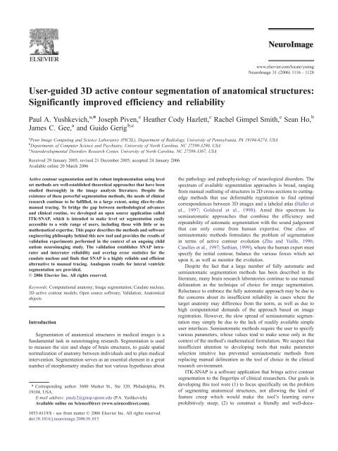
www.elsevier.com/locate/ynimgNeuroImage 31 (2006) 1116 – 1128User-guided 3D active contour segmentation of anatomical structures:Significantly improved efficiency and reliabilityPaul A. Yushkevich, a, * Joseph Piven, c Heather Cody Hazlett, c Rachel Gimpel Smith, c Sean Ho, bJames C. Gee, a and Guido Gerig b,ca Penn Image Computing and Science Laboratory (PICSL), Department of Radiology, University of Pennsylvania, PA 19104-6274, USAb Departments of Computer Science and Psychiatry, University of North Carolina, NC 27599-3290, USAc Neurodevelopmental Disorders Research Center, University of North Carolina, NC 27599-3367, USAReceived 29 January 2005; revised 21 December 2005; accepted 24 January 2006Available online 20 March 2006Active contour segmentation and its robust implementation using levelset methods are well-established theoretical approaches that have beenstudied thoroughly in the image analysis literature. Despite theexistence of these powerful segmentation methods, the needs of clinicalresearch continue to be fulfilled, to a large extent, using slice-by-slicemanual tracing. To bridge the gap between methodological advancesand clinical routine, we developed an open source application calledITK-SNAP, which is intended to make level set segmentation easilyaccessible to a wide range of users, including those with little or nomathematical expertise. This paper describes the methods and softwareengineering philosophy behind this new tool and provides the results ofvalidation experiments performed in the context of an ongoing childautism neuroimaging study. The validation establishes SNAP intraraterand interrater reliability and overlap error statistics for thecaudate nucleus and finds that SNAP is a highly reliable and efficientalternative to manual tracing. Analogous results for lateral ventriclesegmentation are provided.D 2006 Elsevier Inc. All rights reserved.Keywords: Computational anatomy; Image segmentation; Caudate nucleus;3D active contour models; Open source software; Validation; AnatomicalobjectsIntroductionSegmentation of anatomical structures in medical images is afundamental task in neuroimaging research. Segmentation is usedto measure the size and shape of brain structures, to guide spatialnormalization of anatomy between individuals and to plan medicalintervention. Segmentation serves as an essential element in a greatnumber of morphometry studies that test various hypotheses about* Corresponding author. 3600 Market St., Ste 320, Philadelphia, PA19104, USA.E-mail address: pauly2@grasp.upenn.edu (P.A. Yushkevich).Available online on ScienceDirect (www.sciencedirect.com).the pathology and pathophysiology of neurological disorders. Thespectrum of available segmentation approaches is broad, rangingfrom manual outlining of structures in 2D cross-sections to cuttingedgemethods that use deformable registration to find optimalcorrespondences between 3D images and a labeled atlas (Haller etal., 1997; Goldszal et al., 1998). Amid this spectrum liesemiautomatic approaches that combine the efficiency andrepeatability of automatic segmentation with the sound judgementthat can only come from human expertise. One class ofsemiautomatic methods formulates the problem of segmentationin terms of active contour evolution (Zhu and Yuille, 1996;Caselles et al., 1997; Sethian, 1999), where the human expert mustspecify the initial contour, balance the various forces which actupon it, as well as monitor the evolution.Despite the fact that a large number of fully automatic andsemiautomatic segmentation methods has been described in theliterature, many brain research laboratories continue to use manualdelineation as the technique of choice for image segmentation.Reluctance to embrace the fully automatic approach may be due tothe concerns about its insufficient reliability in cases where thetarget anatomy may difference from the norm, as well as due tohigh computational demands of the approach based on imageregistration. However, the slow spread of semiautomatic segmentationmay simply be due to the lack of readily available simpleuser interfaces. Semiautomatic methods require the user to specifyvarious parameters, whose values tend to make sense only in thecontext of the method’s mathematical formulation. We suspect thatinsufficient attention to developing tools that make parameterselection intuitive has prevented semiautomatic methods fromreplacing manual delineation as the tool of choice in the clinicalresearch environment.ITK-SNAP is a software application that brings active contoursegmentation to the fingertips of clinical researchers. Our goals indeveloping this tool were (1) to focus specifically on the problemof segmenting anatomical structures, not allowing the kind offeature creep which would make the tool’s learning curveprohibitively steep; (2) to construct a friendly and well-docu-1053-8119/$ - see front matter D 2006 Elsevier Inc. All rights reserved.doi:10.1016/j.neuroimage.2006.01.015

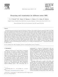
P.A. Yushkevich et al. / NeuroImage 31 (2006) 1116–1128 1119Fig. 2. Examples of edge-based contour evolution before (top) and after (bottom) adding the advection term. Without advection, the contour leaks past theboundaries of the caudate nucleus because the external force is non-negative.as the zeroth level set of some function f, which is defined at everyvoxel in the input image. The relationship N ! ¼ 3/=Ý3/Ý isused to rewrite the PDE (1) as a PDE in /:BBt / ð x;t Þ ¼ F3/: ð5ÞTypically, such equations are not solved over the entire domainof / but only at the set of voxels close to the contour / = 0. SNAPuses the highly efficient Extreme Narrow Banding Method byWhitaker (1998) to solve (5).Software architectureThis section describes SNAP functionality and highlights someof the more innovative elements of its user interface architecture.SNAP was designed to provide a tight but complete set of featuresthat focus on active contour segmentation. It includes tools forviewing and navigating 3D images, manual labeling of regions ofinterest, combining multiple segmentation results, and postprocessingthem in 2D and 3D. Built on the ITK backbone, SNAP canread and write many image formats, and new features can be addedeasily.Image navigation and manual segmentationSNAP’s user interface emphasizes the 3D nature of medicalimages. As shown in Fig. 5a, the main window is divided into fourpanels, three displaying orthogonal cross-sections of the inputimage and the fourth displaying a 3D view of the segmentedstructures. Navigation is aided by a linked 3D cursor whose logicallocation is at the point where the three orthogonal planes intersect.The cursor can be repositioned in each slice view by mousemotion, causing different slices to be shown in the remaining twoslice views. The cursor can also be moved out of the slice planeusing the mouse wheel. This design ensures that the user is alwayspresented with the maximum amount of detail about the voxelunder the cursor and its neighborhood while minimizing theamount of mouse motion needed to navigate through the image.Users can change the zoom in each slice view, and each of the sliceviews can be expanded to occupy the entire program window, asillustrated in Fig. 5b.SNAP provides tools for manual tracing of regions of interest.Internally, SNAP represents labeled regions using an integervalued3D mask image of the same dimensions as the input image.Each voxel in the input image can be assigned a single label or nolabel at all. This approach has the disadvantage that partial volumesegmentations cannot be represented, but it allows users to viewFig. 3. The plot on the left gives an example of three smooth threshold functions with different values of the smoothness parameter j. To the right of the plot arethe input grayscale image and the feature images corresponding to the three thresholds.

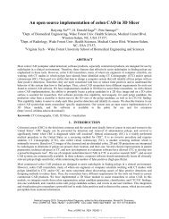
P.A. Yushkevich et al. / NeuroImage 31 (2006) 1116–1128 1121Fig. 6. An example of using cut-plane operations to relabel a segmentation into three components (left lateral ventricle, right lateral ventricle and thirdventricle).live feedback mechanisms. The workflow is divided into threelogical stages.In the first stage, the user chooses between Zhu and Yuille(1996) and Caselles et al. (1997) methods and, depending onthe method chosen, computes the probability map P obj P bg orthe speed function g I . Probability maps are computed, as shownin Fig. 7a, by applying a smooth threshold, which can be onesidedor two-sided, depending on whether the intensity range ofthe structure of interest lies at one of the ends or in the middleof the histogram. Taking advantage of the flexible ITKarchitecture that can apply image processing filters to arbitraryimage subregions, the orthogonal slice views in SNAP provideimmediate feedback in response to changes in parameter values.Alternatively, the user may import an external image, such as atissue class segmentation, as the probability map or speedimage.In the second stage, the user initializes the segmentation byplacing one or more spherical Fseeds_ in the image (Fig. 7b). Theuser can also initialize the active contour with a result of an earliermanual or automatic segmentation. Level set methods allowcontours to change topology, and it is common to place severalseeds within one structure, letting them merge into a single contourover the course of evolution.The last stage of the segmentation workflow is devoted tospecifying the weights of the various terms in the active contourevolution PDE and running the evolution interactively. In orderto accommodate a wider range of users, SNAP provides twoseparate modes for choosing weights. In the casual user mode,weights a, b, and c from the active contour equations aredescribed verbally in terms of their impact on the behavior ofthe evolving contour, accompanied by an interactive, dynamicallyupdated 2D curve evolution illustration that shows theeffect of each of the parameters on the total force acting on theinterface (Fig. 8). The other mode is for users familiar with themathematics of active contours and allows them to specify theweights in a generic evolution formulation that incorporatesboth (2) and (4): F ¼ ah a bh b j ch c 3hI N Y: ð6ÞBy setting h = g I , a =1,b =1,c = 0, the user arrives at theCaselles et al. (1997) formulation, and with h = P obj P bg , a =1,b =0,c = 0, the Zhu and Yuille (1996) formulation is obtained.Formulation (6) corresponds to SNAP’s internal representation ofthe evolution equation.The actual contour evolution is controlled by a VCR-likeinterface. When the user clicks the Fplay_ button, the contourbegins to evolve, and the slice views and, optionally, the 3Dview is updated after each iteration. The user can use Fstop_,Frewind_, and Fsingle step_ buttons to control and terminatecontour evolution. Fig. 9 shows SNAP before and after contourevolution.Before entering the automatic segmentation mode, the usermay choose to restrict segmentation to a 3D region of interestin order to reduce computational cost and memory use. Anoption to resample the region of interest using nearest neighbor,linear, cubic, or windowed sinc interpolation is provided; this isFig. 7. (a) User interface for feature image specification: the user is setting the values of the smooth threshold parameters, and the feature image is displayed inthe orthogonal slice views using a color map. (b) User interface for active contour initialization: the user has placed two spherical bubbles in the caudatenucleus. (For interpretation of the references to colour in this figure legend, the reader is referred to the web version of this article.)

1122P.A. Yushkevich et al. / NeuroImage 31 (2006) 1116–1128Fig. 8. User interface for specifying contour evolution parameters, including the relative weights of the forces acting on the contour. The intuitive interface isshown on the left and the mathematical interface on the right. The parameter specification window also shows how the forces interrelate in a two-dimensionalexample.recommended for images with anisotropic voxels. Whenreturning from automatic mode to the manual mode, SNAPconverts the level set segmentation result to a binary mask andmerges it with the 3D mask image. In the process, the subvoxelaccuracy of the segmentation is compromised. Before merging,the user has the option to export the segmentation as a realvaluedimage.ResultsThe new SNAP tool, with its combination of user-guided 3Dactive contour segmentation and postprocessing via manual tracingin orthogonal slices or using the 3D cut-plane tool, is increasinglyreplacing conventional 2D slice editing for a variety of imagesegmentation tasks. SNAP is used in several large neuroimagingstudies at UNC Chapel Hill, Duke University, and the University ofPennsylvania. Segmentation either uses the soft threshold optionfor the definition of foreground and background, e.g., for thesegmentation of the caudate nucleus in head MRI, or employsexisting tissue probability maps that define object to backgroundprobabilities. This option is used for the segmentation of ventriclesbased on cerebrospinal fluid probabilistic segmentations.An ongoing child neuroimaging autism study serves as atestbed for validation of the new tool as a prerequisite to its use in alarge clinical study. In particular, we chose the segmentation of thecaudate nucleus to establish intrarater and interrater reliability ofapplying SNAP and also to test validity in comparison to manualrater segmentation. The following sections describe validation ofSNAP versus manual rater contour drawing in more details. Inaddition, we provide reliability results for the lateral ventriclesegmentation in SNAP but without a comparison to manualsegmentation.Validation of SNAP: caudate segmentationFrom our partnership with the UNC Psychiatry department, wehave access to a morphologic MRI study with a large set of autisticchildren (N = 56), developmentally delayed subjects (N = 11), andcontrol subjects (N = 17), scanned at age 2. SNAP was chosen asan efficient and reliable tool to segment the caudate nucleus fromhigh-resolution MRI. Before replacing conventional manual outliningby this new tool, we designed a validation study to test thedifference between methods, the difference between operators, andthe variability for each user.Fig. 9. The user interface for contour evolution. The image on the left shows SNAP before evolution is run, and the image on the right is taken after the contourruns for a few seconds. In this example, an edge based feature image is used.

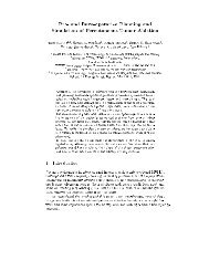
P.A. Yushkevich et al. / NeuroImage 31 (2006) 1116–1128 1123Fig. 10. Two and three-dimensional views of the caudate nucleus. Coronal slice of the caudate: original T1-weighted MRI (left) and overlay of segmentedstructures (middle). Right and left caudate are shown shaded in green and red; left and right putamen are sketched in yellow, laterally exterior to the caudates.The nucleus accumbens is sketched in red outline. Note the lack of contrast at the boundary between the caudate and the nucleus accumbens, and the fine-scalecell bridges between the caudate and the putamen. At right is a 3D view of the caudate and putamen relative to the lateral ventricles. (For interpretation of thereferences to colour in this figure legend, the reader is referred to the web version of this article.)Gray-level MRI dataCaudate segmentation uses high-resolution T1-weighted MRIwith voxel size 0.78 0.78 1.5 mm 3 . The protocol establishedby the UNC autism image analysis group rigidly aligns theseimages to the Talairach coordinate space by specifying anterior andposterior commissure (AC–PC) and the interhemispheric plane.The transformation also interpolates the images to the isotropicvoxel size of 1 mm 3 . Automatic atlas-based tissue segmentationusing EMS (Van Leemput et al., 1999a,b) results in a hardsegmentation and separate probability maps for white matter, graymatter, and cerebrospinal fluid. These three-tissue maps are usedfor SNAP ventricle segmentation, but not for the caudate nucleus,because in some subjects, the intensity distribution of thesubcortical gray matter is different from the cortex.Reliability series and validationFive MRI datasets were arbitrarily chosen from the whole set of100+ images. Data were replicated three times and blinded to forma validation database of 15 images. Three highly trained ratersTable 1Caudate volumes (in mm 3 ) from the validation study comparing SNAPreliability to manual segmentationCase Right caudate volumes Left caudate volumesSNAP Manual SNAP ManualRaterA B A C A B A Cgr1a 3720 3738 3690 3724 3734 3781 3621 3529gr1b 3713 3780 3631 3551 3715 3826 3552 3482gr1c 3790 3786 3735 3749 3758 3790 3521 3510Mean (gr1) 3741 3768 3685 3675 3735 3799 3565 3507gr2a 4290 4353 4267 4120 4087 4141 4137 4262gr2b 4229 4247 4254 4164 4083 4103 4189 4179gr2c 4233 4232 4303 4253 4025 4143 4168 4149Mean (gr2) 4251 4277 4275 4179 4065 4129 4165 4196gr3a 4211 4250 4263 4397 4590 4495 4416 4482gr3b 4289 4155 4221 4149 4562 4506 4444 4417gr3c 4264 4257 4354 4174 4416 4583 4323 4332Mean (gr3) 4255 4221 4279 4240 4523 4528 4394 4410gr4a 4091 4105 4063 4122 3967 4129 4006 4066gr4b 4151 4150 4144 4116 4058 4135 3934 4029gr4c 4081 4149 4103 4037 4081 4141 4001 3995Mean (gr4) 4108 4134 4103 4092 4036 4135 3980 4030gr5a 4112 4197 4167 4125 4355 4295 4278 4321gr5b 4165 4226 4143 4039 4326 4273 4253 4317gr5c 4191 4237 4089 4226 4311 4288 4127 4087Mean (gr5) 4156 4220 4133 4130 4330 4285 4219 4242participated in the validation study; rater A segmented each imagemanually and in SNAP, while rater B only used SNAP and rater Conly performed manual segmentation. Segmentation results betweenpairs of raters or methods were analyzed using commonintraclass correlation statistics (ICC) as well as using overlapstatistics.Caudate nucleus segmentationAt first sight, the caudate seems easy to segment since thelargest fraction of its boundary is adjacent to the lateral ventriclesand white matter. Portions of the caudate boundary can be localizedwith standard edge detection. However, the caudate is also adjacentto the nucleus accumbens and the putamen where there are novisible boundaries in MRI (see Fig. 10). The caudate, nucleusaccumbens, and putamen are distinguishable on histological slides,but not on T1-weighted MRI of this resolution. Another ‘‘troublespot’’for the caudate is where it borders the putamen; there are‘‘fingers’’ of cell bridges adjacent to blood vessels which span thegap between the two.Manual boundary drawingUsing the drawing tools in SNAP, we have developed a highlyreliable protocol for manual caudate segmentation using slice-bysliceboundary drawing in all three orthogonal views. In addition toboundary overlays, the segmentation is supported by a 3D displayof the segmented structure. The coupling of cursors between 2Dslices and the 3D display help significantly reduce slice-by-slicejitter that is often seen in this type of segmentations. SegmentationTable 2Intrarater and interrater reliability of caudate segmentationValidation type Side Intra A Intra B Intra AB Inter ABIntra-/interrater manual Right 0.963 0.845 0.902 0.916(A Manual, B Manual) Left 0.970 0.954 0.961 0.967Manual vs. SNAP Right 0.963 0.967 0.964 0.967(A Manual, B SNAP) Left 0.970 0.969 0.969 0.907Intra-/interrater SNAP(A SNAP, B SNAP)Right 0.967 0.958 0.962 0.958Left 0.969 0.990 0.978 0.961Reliability was measured based on 3 replications of 5 test datasets by tworaters. Reliability values for (1) manual segmentation by two experts; (2)manual vs. SNAP segmentation by the same expert; and (3) SNAPsegmentation by two experts show the excellent reliability of both methodsand the excellent agreement between manual expert’s segmentation andSNAP. SNAP reduced segmentation time from 1.5 h to 30 min, while thetraining period to establish reliability was several months for the manualmethod and significantly shorter for SNAP.

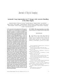
1124P.A. Yushkevich et al. / NeuroImage 31 (2006) 1116–1128Table 3Overlap statistics between pairs of caudate segmentations, categorized bydifferent methods and ratersCategory l Left r Left l Right r Right n1. SNAP A vs. SNAP A 97.5 0.836 97.7 0.598 152. SNAP B vs. SNAP B 98.8 0.291 98.7 0.679 153. SNAP intrarater average 98.1 0.931 98.2 0.823 304. SNAP A vs. SNAP B 97.3 0.810 97.5 0.686 455. Manual A vs. Manual A 94.0 0.802 94.2 0.617 156. Manual C vs. Manual C 93.4 0.568 93.1 0.504 157. Manual intrarater average 93.7 0.752 93.6 0.783 308. Manual A vs. Manual C 92.5 0.913 91.9 0.697 459. SNAP A vs. Manual A 92.2 0.991 92.6 0.515 4510. SNAP A vs. Manual C 91.3 0.602 91.0 0.893 4511. SNAP B vs. Manual A 91.9 1.11 92.5 0.421 4512. SNAP B vs. Manual C 91.2 0.635 91.1 0.733 4513. SNAP vs. Manual 91.5 0.860 91.5 0.999 135interrater averageLetters A, B, and C refer to individual raters. Overlap values are given inpercent, i.e., overlap (S 1 , S 2 ) = 100%*DSC (S 1 , S 2 ). The number of pairs ineach category is given in the last column (n).time for left and right caudate is approximately 1.5 h forexperienced experts.3D active contour segmentationWe developed a new segmentation protocol for caudatesegmentation based on the T1 gray level images with emphasison efficiency and optimal reliability. The caudate nucleus is asubcortical gray matter structure. T1 intensity values of thecaudate regions in the infant MRI showed significant differencesamong subjects and required individual adjustment. We placesample regions in four axial slices of the caudate, measure theintensity and standard deviation of the sample regions, then usethose values to guide the setting of the upper and lowerthresholds in the preprocessing step of SNAP. This results inforeground/background maps which guide the level set evolution.Parameters for smoothness and speed were trained in apilot study and were kept constant for the whole study. Thesame regions were used as initialization regions. Evolution wasstopped after the caudate started to bleed into the adjacentputamen. Optimal intensity window selection and active contourevolution take only about 5 min for the left and right caudate.In some caudate segmentation protocols, the inferior boundaryis cut off by the selection of an axial cut plane, which onlytakes a few additional seconds using the cut-plane feature inSNAP. In our autism project, we decided to add a preciseseparation from the putamen and a masking of the left and rightnucleus accumbens. This is a purely manual operation sincethere are no visible boundaries between caudate and nucleusaccumbens in the MR image. This step added another 30 minto the whole process. The total segmentation time was reducedfrom originally 1.5 h for slice-by-slice contour drawing to 35min, with the option to be reduced to only 5 min if simple cutplanesfor inferior boundaries would be sufficient for the giventask, which is similar to the protocol applied by Levitt et al.(2002). The raters also reported that they felt much morecomfortable with the SNAP tool since they could focus theireffort on a small part of the boundary that is most difficult totrace.Volumetric analysisTable 1 lists the left and right caudate volumes for manualsegmentation (slice by slice contouring) and user-assisted 3Dactive contour segmentation (SNAP). Results of the reliabilityanalysis using one-way random effects intraclass correlationstatistics (Shrout and Fleiss, 1979) are shown in Table 2.The table shows not only the excellent reliability of SNAPsegmentation but also reflects the excellent reliability of themanual experts trained over several months. Therefore, reliabilitybetween methods is not significantly different. On the basisof volume comparisons, the SNAP segmentation, which requiresmuch less training and is significantly more efficient, is shownequivalent to the manual expert, both with respect to intramethodreliability and intermethod validity. However, this is tobe compared with the significantly reduced segmentation timeand short rater training time of SNAP.Overlap analysisIn addition to volume-based reliability analysis, we compareSNAP and manual methods in terms of overlap between differentsegmentations of each instance of the caudate. Overlap is a moreaccurate measure of agreement between two segmentations thanvolume difference because the latter may be zero for twocompletely different segmentations. For every subject–caudatecombination, we measure the overlap between all ordered pairs ofavailable segmentations. There are 10 structures (5 subjects, leftand right), and for each structure, there are 12 differentFig. 11. Box and whisker plots showing order statistics (minimum, 25% quantile, median, 75% quantile, maximum) of overlaps between pairs of segmentationsof the caudate nucleus. The horizontal axis represents 13 different categories of pairwise comparisons that are listed in Table 3, and the vertical axis plots theDice Similarity Coefficient (DCS). Columns 1–4 are SNAP-to-SNAP comparisons, columns 5–8 are manual-to-manual comparisons, and columns 9 – 13 aremixed-method comparisons. Orange boxes represent intrarater comparisons for specific raters; red boxes stand for intrarater comparisons pooled over availableraters; light blue boxes are interrater comparisons for specific pairs of raters; and dark blue boxes are interrater comparisons pooled over available rater pairs.(For interpretation of the references to colour in this figure legend, the reader is referred to the web version of this article.)

P.A. Yushkevich et al. / NeuroImage 31 (2006) 1116–1128 1125 12segmentations (2 raters, 2 methods, 3 repetitions) and ¼26 ordered pairs. For each pair, we count the number 2 of voxels inthe input image that belong to both segmentations. Following thestatistical approach described in (Zou et al., 2004), we define theoverlap between segmentations S 1 and S 2 as the Dice SimilarityCoefficient (DSC):DSCðS 1 ; S 1 Þ ¼ 2Vol ð S 17S 2 ÞVolðS 1 ÞþVolðS 2 Þ : ð7ÞThis symmetric measure of segmentation agreement lies in therange [0, 1], with larger values indicating greater overlap.Table 3 lists means and standard deviations of the overlaps forthe left and right caudate within 13 different categories ofcomparisons. These categories fall into three larger classes:SNAP-to-SNAP comparisons (i.e., pairs where both segmentationswere generated with SNAP), manual-to-manual comparisons, andmixed SNAP-to-manual comparisons. Within each class, categoriesinclude (1) all pairs where both segmentations were performed by agiven rater, (2) all pairs where both segmentations were performedby the same rater, and (3) all pairs where segmentations wereperformed by different raters. Fig. 11 displays box and whisker plotsof the same 13 categories. It is immediately noticeable that thecomparisons in the SNAP-to-SNAP group yield significantly betteroverlaps than other types of comparisons; in fact, the worst overlapbetween any pair of SNAP segmentations is still better than the bestoverlap between any pair of manual segmentations or any pair whereboth methods are used. This indicates that SNAP caudatesegmentation exhibits significantly better repeatability than manualsegmentation.To confirm this finding quantitatively, we perform an ANOVAexperiment adopted from Zou et al. (2004), who studied repeatabilityin the context of pre- and postoperative prostate segmentation.Variance components in the ANOVA model include the method(M Z {SNAP, Manual}), case (i.e., subject; C Z {1, 2, 3, 4, 5}),anatomy A Z {l. caudate, r. caudate}, and repetition pair P Z {(a,b), (b, c), (a, c)}, i.e., one of the three possible ordered pairs ofsegmentations performed by a given rater in a given case on a givenstructure (symbols a, b, c correspond to the order in which the raterperformed the segmentations). Zou et al. (2004) pools the modelover all raters, but in our case, since only rater A performedsegmentation using both methods, we just include segmentations byrater A in the model. Following Zou et al. (2004), the modelincludes two interaction terms: M S and C S, and the outcomeTable 4Results of ANOVA experiment to determine whether segmentationrepeatability measured in terms of overlap varies according to method(M), rater (R), case (C), anatomical structure (A) or the pair ofsegmentations involved in the overlap computation ( P)VariancecomponentsD.o.F.SumsquareMeansquareF statisticsP valueMethod (M) 1 13.886 13.886 220.639 –Segmentation 2 0.027 0.013 0.214 0.808pair ( P)Case (C) 4 0.759 0.190 3.015 0.029Anatomical 1 0.033 0.033 0.520 0.475structure (A)M P 2 0.117 0.059 0.931 0.402C P 8 0.167 0.021 0.337 0.947Residuals 41 2.580 0.063 – –Table 5Ventricle volumes (in mm 3 ) from the SNAP reliability experimentCase Left Right Case Left RightA B A B A B A Bgr1a 2935 2942 3375 3389 gr4a 1605 1581 1719 1752gr1b 2954 2953 3363 3404 gr4b 1578 1605 1719 1725gr1c 2955 2936 3380 3386 gr4c 1606 1607 1719 1725Mean 2948 2944 3373 3393 Mean (gr4) 1596 1598 1719 1734(gr1)gr2a 5565 5572 6833 6824 gr5a 3687 3562 7776 7436gr2b 5561 5579 6825 6830 gr5b 4178 3511 7725 7541gr2c 5564 5577 6830 6824 gr5c 3871 3561 7758 7389Mean 5563 5576 6829 6826 Mean (gr5) 3912 3544 7753 7455(gr2)gr3a 2775 2781 6778 6963gr3b 2682 2780 7307 6971gr3c 2734 2772 7217 6982Mean 2730 2778 7101 6972(gr3)Five test cases, replicated three times (column one) have been segmented bytwo raters (A, B), who were blinded to the cases.variable is derived by standardizing the DSC using the logittransform:DSCðS 1 ; S 2 ÞLDSCðS 1 ; S 2 Þ ¼ lnð8Þ1 DSCðS 1 ; S 2 ÞOur ANOVA results are listed in Table 4. We conclude thatSNAP segmentations are significantly more reproducible thanmanual segmentation ( F = 1066, P b 0.001). We observe asignificant effect of case on repeatability ( F = 5.176, P = 0.001),implying that reproducibility varies by subject. There is no evidenceto support the hypothesis that repeatability improves with training,as the choice of repetition pair has no significant effect on theoverlap ( P = 0.287). We also do not find a significant difference inrepeatability between left and right caudates. A limitation of theabove analysis is that segmentations from only one rater are includedin the ANOVA. The other two raters could not be included becauserater B used SNAP for all caudate segmentations, and allsegmentations by rater C were manual. A stronger case could havebeen made if each of these raters had used both methods, allowing usto treat rater as a random effect. However, visual analysis of boxplots in Fig. 11 suggests that while repeatability varies by raterwithin each method, this difference is smaller than the overalldifference in repeatability between the methods.Lateral ventricle segmentationUnlike the caudate, which has a simple shape but lacks clearlydefined MRI intensity boundaries, the lateral ventricles are complexgeometrically yet have an easily identifiable boundary. To demonstratethe breadth of SNAP segmentation, we present the results of aTable 6Intrarater and interrater reliability of lateral ventricle segmentation in SNAPValidation type Side Intra A Intra B Intra AB Inter ABIntra-/interrater SNAP Right 0.9942 0.9999 0.9970 0.9917(A SNAP, B SNAP) Left 0.9977 0.9998 0.9987 0.9976Reliability was measured based on 3 replications of 5 test datasets by tworaters.

1126P.A. Yushkevich et al. / NeuroImage 31 (2006) 1116–1128Table 7Overlap statistics for left and right lateral ventricle segmentationsCategory l Left s Left l Right s Right n1. SNAP A vs. SNAP A 99.5 0.481 99.5 0.482 152. SNAP B vs. SNAP B 99.0 1.16 98.6 1.69 153. SNAP intrarater average 99.3 0.898 99.1 1.31 304. SNAP A vs. SNAP B 98.9 0.914 98.3 2.20 45Overlap values are given as percentages, i.e., overlap (S 1 , S 2 ) = 100%*DSC(S 1 , S 2 ).repeatability experiment for lateral ventricle segmentation. As forthe caudate, we randomly selected five MRI images from the childautism database and applied our standard image processing pipeline,including tissue class segmentation using EMS. Our ventriclesegmentation protocol involves placing three initialization seeds ineach ventricle and running the active contour segmentation untilthere is no more expansion into the horns. Afterwards, the 3D cutplanetool is used to separate the left ventricle from the right. In somecases, active contour segmentation will bleed into the third ventricle,which can be corrected using the cut-plane tool or by slice-by-sliceediting. If the ventricles are very narrow, the evolving interface maynot reach the inferior horns, and there also are rare cases where partsof the ventricles are so narrow that they are misclassified by EMS.These problems are corrected by postprocessing, which involvesreapplying active contour segmentation to the trouble regions orcorrecting the segmentation manually. Nevertheless, the approximateaverage time to segment a pair of lateral ventricles is 15 min,including initialization, running the automatic pipeline, reviewing,and editing.Using SNAP, each of the five selected images was segmentedthree times by two blinded raters; in contrast to caudate validation,manual segmentation was not performed. The volumes of theventricle segmentations are listed in Table 5, and the volume-basedreliability statistics are given in Table 6. SNAP interrater reliabilitycoefficients exceed 0.99 for both ventricles, matching the reliabilityof manual segmentation, as reported by Blatter et al. (1995).Overlap statistics are summarized in Table 7 and Fig. 12. Despitethe ventricles’ complex shape, the average DSC values (0.989 forthe left ventricle and 0.983 for the right) are higher than for caudatesegmentation.DiscussionThe caudate segmentation validation, which compares theSNAP tool to manual segmentation by highly trained raters,demonstrates the excellent reliability of the tool for efficient threedimensionalsegmentation. While the volume-based reliabilityanalysis shows a similar range of intramethod reliability for bothsegmentation approaches, overlap analysis reveals that SNAPsegmentation exhibits significantly improved repeatability. SNAPcut the segmentation time by a factor of three and also significantlyreduced the training time to establish expert reliability. Besidesrepeatability and efficiency, our experts preferred using SNAP overslice contouring due to the tool’s capability to display 3Dsegmentations in real time and due to the simple option topostprocess the automated segmentation using 3D tools.In addition to brain structure extraction in MRI, SNAP hasfound a variety of uses in other imaging modalities and anatomicalregions. For example, in radiation oncology applications, SNAPhas proven useful for segmenting the liver, kidneys, bonystructures, and tumors in thin-slice computer tomography (CT)images. In emphysema research involving humans and mice,SNAP has been used to extract lung cavities in CT, as well aspulmonary vasculature in MRI. SNAP has also proven invaluableas a supporting tool for developing and validating medical imageanalysis methodology. It has found countless uses in our ownlaboratories, such as to postprocess the results of automatic brainextraction, to identify landmarks that guide image registration andto build anatomical atlases for template deformation morphology(Yushkevich et al., 2005).Despite SNAP’s versatility, its automatic segmentation pipelineis limited to a specific subset of segmentation problems where thestructure of interest has a different intensity distribution from mostof the surrounding tissues. Future development of SNAP will focuson simplifying the segmentation of structures whose intensitydistribution is indistinguishable from some of its neighbors. Thiswill be accomplished by (1) preventing the evolving interface fromentering certain regions via special seeds placed by the user, whichpush back on the interface, similar to the ‘‘volcanoes’’ in theseminal paper by Kass et al. (1988), and (2) providing additional3D postprocessing tools that will make it easier to cut away parts ofthe interface that has leaked. These postprocessing tools will bebased on graph-theoretic algorithms. One such tool will allow theuser to trace a closed path on the surface of the segmentation result,after which the minimal surface bounded by that path will becomputed and used to partition the segmentation in two. Anotherfuture feature of SNAP will be an expanded user interface fordefining object and background probabilities in the Zhu and Yuille(1996) method, where the user will be able to place a number ofsensors inside and outside of the structure in order to estimate theintensity distribution within the structure. In order to account forintensity inhomogeneity in MRI, SNAP will include an option tolet the estimated distribution vary spatially. Finally, we plan toFig. 12. Box and whisker plots of overlaps between pairs of segmentations of the lateral ventricles nucleus. All columns represent SNAP-to-SNAPcomparisons; columns 1 and 2 represent intrarater comparisons for specific raters; column 3 plots intrarater comparisons pooled over the two raters; and column4 shows interrater comparisons.

P.A. Yushkevich et al. / NeuroImage 31 (2006) 1116–1128 1127tightly integrate SNAP will external tools for brain extraction,tissue class segmentation, and inhomogeneity field correction.ConclusionITK-SNAP is an open source medical image processingapplication that fulfills a specific and pressing need of biomedicalimaging research by providing a combination of manual andsemiautomatic tools for extracting structures in 3D image data ofdifferent modalities and from different anatomical regions.Designed to maximize user efficiency and to provide a smoothlearning curve, the user interface is focused entirely on segmentation,parameter selection is simplified using live feedback, andthe number of features unrelated to segmentation kept to aminimum. Validation in the context of caudate nucleus and lateralventricle segmentation in child MRI demonstrates excellentreliability and high efficiency of 3D SNAP segmentation andprovides strong motivation for adopting SNAP as the segmentationsolution for clinical research in neuroimaging and beyond.AcknowledgmentsThe integration of the SNAP tool with ITK was performed byCognitica Corporation under NIH/NLM PO 467-MZ-202446-1.The validation study is supported by the NIH/NIBIB P01EB002779, NIH Conte Center MH064065, and UNC NeurodevelopmentalDisorders Research Center, Developmental NeuroimagingCore. The MRI images of infants and expert manualsegmentations are funded by NIH RO1 MH61696 and NIMH MH64580 (PI: Joseph Piven). Manual segmentations for the caudatestudy were done by Michael Graves and Todd Mathews; SNAPcaudate segmentation was performed by Rachel Smith and MichaelGraves; Rachel Smith and Carolyn Kylstra were raters for theSNAP ventricle segmentation.Many people have contributed to the development of ITK-SNAP and its predecessors: Silvio Turello, Joachim Schlegel,Gabor Szekely (ETH Zurich, Original AVS Module), Sean Ho,Chris Wynn, Arun Neelamkavil, David Gregg, Eric Larsen, SanjaySthapit, Ashraf Farrag, Amy Henderson, Robin Munesato, MingYu, Nathan Moon, Thorsten Scheuermann, Konstantin Bobkov,Nathan Talbert, Yongjik Kim, Pierre Fillard (UNC Chapel Hillstudent projects, 1999- 2003, supervised by Guido Gerig), DanielS. Fritsch and Stephen R. Aylward (ITK Integration, 2003–2004).Special thanks are extended to Terry S. Yoo, Joshua Cates, LuisIba|ñez, Julian Jomier, and Hui Zhang.ReferencesAlsabti, Ranka, Singh, 1998. An efficient parallel algorithm for highdimensional similarity join. IPPS: 11th International Parallel ProcessingSymposium. IEEE Computer Society Press.Avants, B., Schoenemann, P., Gee, J., in press. Lagrangian framediffeomorphic image registration: Morphometric comparison of humanand chimpanzee cortex. Med. Image Anal. (Available online 3 June2005).Blatter, D.D., Bigler, E.D., Gale, S.D., Johnson, S.C., Anderson, C.V.,Burnett, B.M., Parker, N., Kurth, S., Horn, S.D., 1995. Quantitativevolumetric analysis of brain MR: normative database spanning 5decades of life. AJNR Am. J. Neuroradiol. 16 (2), 241–251.Caselles, V., Catte, F., Coll, T., Dibos, F., 1993. A geometric model foractive contours. Numer. Math. 66, 1 –31.Caselles, V., Kimmel, R., Sapiro, G., 1997. Geodesic active contours. Int. J.Comput. Vis. 22, 61–79.Cootes, T., Edwards, G., Taylor, C., 1998. Active appearance models.European Conference on Computer Vision, vol. 2. Freiburg, Germany,pp. 484–498.Davatzikos, C., Genc, A., Xu, D., Resnick, S.M., 2001. Voxel-basedmorphometry using the ravens maps: methods and validation usingsimulated longitudinal atrophy. NeuroImage 14 (6), 1361– 1369.Davies, R.H., Twining, C.J., Cootes, T.F., Waterton, J.C., Taylor, C.J., 2002.A minimum description length approach to statistical shape modeling.IEEE Trans. Med. Imag. 21 (5), 525–537.Gering, D., Nabavi, A., Kikinis, R., Hata, N., Odonnell, L., Grimson,W.E.L., Jolesz, F., Black, P., Wells III, W.M., 2001. An integratedvisualization system for surgical planning and guidance using imagefusion and an open MR. J. Magn. Reson. Imaging 13, 967–975.Goldszal, A., Davatzikos, C., Pham, D.L., Yan, M.X.H., Bryan, R.N.,Resnick, S.M., 1998. An image processing system for qualitative andquantitative volumetric analysis of brain images. J. Comput. Assist.Tomogr. 22 (5), 827–837.Gurleyik, K., Haacke, E.M., 2002. Quantification of errors in volumemeasurements of the caudate nucleus using magnetic resonanceimaging. J. Magn. Reson. Imaging 15 (4), 353–363.Haller, J., Banerjee, A., Christensen, G., Gado, M., Joshi, S., Miller, M.,Sheline, Y., Vannier, M., Csernansky, J., 1997. Three-dimensionalhippocampal MR morphometry by high-dimensional transformation ofa neuroanatomic atlas. Radiology 202, 504–510.Hokama, H., Shenton, M.E., Nestor, P.G., Kikinis, R., Levitt, J.J., Metcalf,D., Wible, C.G., O’Donnell, B.F., Jolesz, F.A., McCarley, R.W., 1995.Caudate, putamen, and globus pallidus volume in schizophrenia: aquantitative MRI study. Psychiatry Res. 61 (4), 209–229.Ibanez, L., Schroeder, W., Ng, L., Cates, J., 2003. The ITK Software Guide.Kitware, Inc.Joshi, S., Miller, M.I., 2000. Landmark matching via large deformationdiffeomorphisms. IEEE Trans. Image Process. 9 (8), 1357–1370.Joshi, S., Pizer, S., Fletcher, P., Yushkevich, P., Thall, A., Marron, J., 2002.Multi-scale deformable model segmentation and statistical shape analysisusing medial descriptions. IEEE Trans. Med. Imag. 21 (5), 538–550.Kass, M., Witkin, A., Terzopoulos, D., 1988. Snakes: active contourmodels. Int. J. Comput. Vis. 1 (4), 321–331.Keshavan, M.S., Rosenberg, D., Sweeney, J.A., Pettegrew, J.W., 1998.Decreased caudate volume in neuroleptic-naive psychotic patients. Am.J. Psychiatry 155 (6), 774–778.Lefohn, A.E., Cates, J.E., Whitaker, R.T., 2003. Interactive, GPU-basedlevel sets for 3d segmentation. Medical Image Computing andComputer-assisted, pp. 564–572.Levitt, J.J., McCarley, R.W., Dickey, C.C., Voglmaier, M.M., Niznikiewicz,M.A., Seidman, L.J., Hirayasu, Y., Ciszewski, A.A., Kikinis, R., Jolesz,F.A., Shenton, M.E., 2002. MRI study of caudate nucleus volume and itscognitive correlates in neuroleptic-naive patients with schizotypalpersonality disorder. Am. J. Psychiatry 159 (7), 1190–1197.Lorensen, W.E., Cline, H.E., 1987. Marching cubes: a high resolution 3Dsurface construction algorithm. Comput. Graph. 21 (4), 163–169.McAuliffe, M.J., Lalonde, F.M., McGarry, D., Gandler, W., Csaky, K., Trus,B.L., 2001. Medical image processing, analysis and visualization inclinical research. CBMS ’01: Proceedings of the Fourteenth IEEESymposium on Computer-Based Medical Systems. IEEE ComputerSociety, Washington, DC, USA, p. 381.Naismith, S., Hickie, I., Ward, P.B., Turner, K., Scott, E., Little, C.,Mitchell, P., Wilhelm, K., Parker, G., 2002. Caudate nucleus volumesand genetic determinants of homocysteine metabolism in the predictionof psychomotor speed in older persons with depression. Am. J.Psychiatry 159 (12), 2096–2098.Osher, S., Sethian, J., 1988. Fronts propagating with curvature speed:algorithms based on Hamilton-Jacobi formulations. J. Comput. Phys.79, 12–49.

1128P.A. Yushkevich et al. / NeuroImage 31 (2006) 1116–1128Robb, R.A., Hanson, D.P., 1995. The ANALYZE (tm) software system forvisualization and analysis in surgery simulation. In: Lavallé, S., Taylor,R., Burdea, G., Mösges, R. (Eds.), Computer Integrated Surgery. MITPress, pp. 175–190.Schroeder, W.J., Martin, K.M., Lorensen, W.E., 1996. The design andimplementation of an object-oriented toolkit for 3D graphics andvisualization. In: Yagel, R., Nielson, G.M. (Eds.), IEEE Visualization’96, pp. 93–100.Sethian, J.A., 1999. Level Set Methods and Fast Marching Methods.Cambridge Univ. Press.Shrout, P., Fleiss, J., 1979. Intraclass correlations: uses in assessing raterreliability. Psychol. Bull. 86, 420–428.Thirion, J.-P., 1996. Non-rigid matching using demons. CVPR ’96: Proceedingsof the 1996 Conference on Computer Vision and Pattern Recognition(CVPR ’96). IEEE Computer Society, p. 245 (0-8186-7258-7).Van Leemput, K., Maes, F., Vandermeulen, D., Suetens, P., 1999a.Automated model-based bias field correction of MR images of thebrain. IEEE Trans. Med. Imag. 18, 885–896.Van Leemput, K., Maes, F., Vandermeulen, D., Suetens, P., 1999b.Automated model-based tissue classification of MR images of thebrain. IEEE Trans. Med. Imag. 18, 897–908.Wells, W.M. III, Grimson, W.E.L., Kikinis, R., Jolesz, F.A., 1995. Adaptivesegmentation of MRI data. In: Ayache III, N. (Ed.), Computer Vision,Virtual Reality and Robotics in Medicine. Springer-Verlag.Whitaker, R.T., 1998. A level-set approach to 3d reconstruction from rangedata. Int. J. Comput. Vis. 29 (3), 203–231 (ISSN 0920-5691).Yushkevich, P.A., Dubb, A., Xie, Z., Gur, R., Gur, R., Gee, J.C.,2005. Regional structural characterization of the brain of schizophreniapatients. Acad. Radiol. 12 (10), 1250–1261.Zhu, S.C., Yuille, A., 1996. Region competition: unifying snakes, regiongrowing, and Bayes/mdl for multiband image segmentation. IEEE Trans.Pattern Anal. Mach. Intell. 18 (9), 884–900 (ISSN 0162-8828).Zou, K.H., Warfield, S.K., Bharatha, A., Tempany, C.M.C., Kaus, M.R.,Haker, S.J., Wells III, W.M., Jolesz, F.A., Kikinis, R., 2004. Statisticalvalidation of image segmentation quality based on a spatial overlapindex. Acad. Radiol. 11 (2), 178–189.