Modeling Tools for Environmental Engineers and Scientists

More documents

Recommendations

Info

On substituting for g and j from the above, C 0 = W/αQ, where W is the massrate of discharge into the river. The final model for this problem is, therefore:Step 4: Interpretation of ResultsC = αWQ e gx for x ≤ 0 (2.26)C = αWQ e jx for x ≥ 0 (2.27)The calibration and validation of the model will be highly problemspecific.Initial interpretations can include simulations, sensitivity analysis,and comparison with other similar systems. As a first step in this case, themodel can be run with typical parameters and known inputs. The output canbe used to corroborate the performance of the model against intuition, pastexperience, or literature results to verify that the model outputs generally followthe observed profiles and are within reasonable ranges. Because the resultin this case is a function of x rather than a numerical value, it may be usefulto plot the variation of C as a function of x to check if the model is reflectingthe spatial concentration profile.As an example of calibration and validation, let us use an artificial data set(adapted from Thomann and Mueller, 1987):Distance (mi) –15 –10 –5 0 5 10 15Concentration (mg/L) 0.43 1.22 3.50 10.00 4.49 2.02 0.91This data set had been collected on an estuary flowing at 100 cfs with an averagecross-sectional area of 10 × 10 5 sq ft, receiving a waste input of 372,000lbs/day at 0 miles. The decay rate of the waste material was measured to be0.1 day –1 . The dispersion for this estuary was estimated to be in the range of2–5 sq miles/day.As a first step, an appropriate value for the dispersion coefficient, E, hasto be established. The data from the upstream portion of the estuary are usedto calibrate the model to fit the four data points by running the model withvarious values of E ranging from 2 to 5 sq miles/day. Given the value of E,the remaining three data points may be used to validate the model. These considerationsare illustrated in Figure 2.8, from which the value of E can be estimatedto be 3 sq miles/day. With this value for E, the model is capable offitting the upstream data points as well as predicting the downstream datapoints. While acknowledging that the validation and calibration exercise inthis example is somewhat academic, the very same procedure is used in practiceto calibrate and validate mathematical models.© 2002 by CRC Press LLC
Figure 2.8 Model predictions vs. measured data.The value of the simplifying assumptions made at the beginning of theanalysis is in the reduction of the governing equation to a form amenable toa closed solution. Such an analysis provides highly useful insight and acts asa stepping stone for the modeler to gradually add pertinent details andrefinements to build more realistic models. Needless to say, as the modelsbecome more detailed and realistic, analytical methods of solving the governingequations can be extremely complicated or impossible. In such cases,using computer-based, numerical approaches is the only way to complete themodeling process. In the next chapter, some of the common analytical andnumerical approaches used in environmental modeling efforts will be reviewed.© 2002 by CRC Press LLC
Page 2: © 2002 by CRC Press LLCModeling To
Page 5 and 6: ContentsPrefaceAcknowledgmentsFUNDA
Page 7 and 8: APPLICATIONS8. MODELING OF ENGINEER
Page 9 and 10: The contents of this book are organ
Page 11 and 12: PART IFundamentals© 2002 by CRC Pr
Page 13 and 14: The models resulting from the model
Page 15 and 16: within the grasp of only a few with
Page 17 and 18: 1.2.3 STATIC VS. DYNAMICWhen a syst
Page 19 and 20: Real SystemsMathematical ModelsDete
Page 21 and 22: through several pathways. Consequen
Page 23 and 24: ange of complex environmental appli
Page 25 and 26: APPENDIX 1.1 TYPICAL USES OF MATHEM
Page 27 and 28: APPENDIX 1.2 (continued)Target Audi
Page 29 and 30: characteristics. The system is isol
Page 31 and 32: formation, inferencing, testing, va
Page 33 and 34: system-surroundings interactions ca
Page 35 and 36: 2.2.4 INTERPRETATION AND EVALUATION
Page 37 and 38: to fill in where scientific theorie
Page 39 and 40: Figure 2.3 Schematic of real system
Page 41 and 42: Table 2.1 Variables, Symbols, Dimen
Page 43 and 44: ∴Net diffusive inflow = -EA ∂
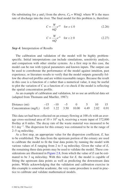
Page 45: in terms of the model parameters al
Page 49 and 50: variables. Deterministic systems ca
Page 51 and 52: e possible, and a computational met
Page 53 and 54: or, in matrix forma 11 a 12 a 13a 2
Page 55 and 56: (a)(b)Figure 3.3 (a) Setting up Sol
Page 57 and 58: Figure 3.5 Using MATLAB ® for solv
Page 59 and 60: Another method, known as the Newton
Page 61 and 62: and so on up tof n (x 1 , x 2 , . .
Page 63 and 64: c. Second-order equation with equid
Page 65 and 66: Figure 3.9 Solution of ODE by Mathe
Page 67 and 68: over the entire step, which may be
Page 69 and 70: Hence, the original problem is now
Page 71 and 72: 2∂ f f i1,j1 - f i-1,j1 - f i1,j-
Page 73 and 74: modeling, in diagnosis and troubles
Page 75 and 76: For the reach x ≥ a: C S D K
Page 77 and 78: contaminants that do not undergo an
Page 79 and 80: known as an intensive property. Oth
Page 81 and 82: Dissolved mass in sample = dissolve
Page 83 and 84: Figure 4.2 Illustration of steady s
Page 85 and 86: 4.3.2.2 Dalton’s LawDalton’s La
Page 87 and 88: Table 4.2 Different Forms of Quanti
Page 89 and 90: M olesoxygenHence, K a-w = = 8 - 3
Page 91 and 92: SolutionThe flux, N, which is the d
Page 93 and 94: Figure 4.3 Illustration of the Two-
Page 95 and 96: where C s is the concentration of t
Page 97 and 98:
Fraction in dissolved form = f d =
Page 99 and 100:
in the air (M/L -3 ), C a is the co
Page 101 and 102:
ackward reactions can expressed in
Page 103 and 104:
4.7.2 ELEMENTARY REACTIONSThe rate
Page 105 and 106:
excess energy. The direct photolysi
Page 107 and 108:
4.8 MATERIAL BALANCEAs indicated in
Page 109 and 110:
SolutionLet M be the mass of chemic
Page 111 and 112:
CpHence, the final result isEXERCIS
Page 113 and 114:
APPENDIX 4.1 COMMON PARTITION COEFF
Page 115 and 116:
analyzing and modeling them. The ex
Page 117 and 118:
\5.2.2 HETEROGENEOUS REACTORSHetero
Page 119 and 120:
CC = in -(t t 0 )k C t in0 k- C
Page 121 and 122:
Worked Example 5.1A wastewater trea
Page 123 and 124:
or,C L = C 0 e -(k /u)L = C 0 e -k
Page 125 and 126:
HRT = 1 k (1 - )The overall HRT
Page 127 and 128:
The MB equation for the above syste
Page 129 and 130:
the particle surface (ML -2 T -1 ),
Page 131 and 132:
0 = QX - Q(X - dX) - K L (aAdz)(X -
Page 133 and 134:
chemical engineering applications.
Page 135 and 136:
This expression does not provide an
Page 137 and 138:
If the WWTP used air instead of pur
Page 139 and 140:
and degradation of the natural envi
Page 141 and 142:
The solution to the above PDE gives
Page 143 and 144:
• river 2: x = 15000.5 dmay ∴u
Page 145 and 146:
These functions are valuable tools
Page 147 and 148:
this problem. Once the basic “syn
Page 149 and 150:
giving the condition Q > 4πRu for
Page 151 and 152:
directions, and the last term repre
Page 153 and 154:
SolutionTo be conservative, it may
Page 155 and 156:
zone, because the hydraulic conduct
Page 157 and 158:
6.2.5 FLOW OF AIR AND CONTAMINANTS
Page 159 and 160:
time-dependent volumetric flow rate
Page 161 and 162:
Solution(1) The steady state concen
Page 163 and 164:
As a first step in modeling a river
Page 165 and 166:
where a 1,4 is the conversion facto
Page 167 and 168:
© 2002 by CRC Press LLCFigure 6.8
Page 169 and 170:
Figure 6.106.5 Consider the stream
Page 171 and 172:
Case 4: Pulse Source in Two Dimensi
Page 173 and 174:
End users often adapted these model
Page 175 and 176:
to further enhance the capabilities
Page 177 and 178:
are always expressed in the standar
Page 179 and 180:
know the program’s environment. M
Page 181 and 182:
typing in the equations in algebrai
Page 183 and 184:
accessed in Simulink ® models. The
Page 185 and 186:
By combining the above simple funct
Page 187 and 188:
Concentration [mg/L]Figure 7.3 Lake
Page 189 and 190:
saving considerable model building
Page 191 and 192:
dependent variable, the dependent v
Page 193 and 194:
command is used to keep the plot fr
Page 195 and 196:
Figure 7.10 Lake problem solved wit
Page 197 and 198:
simulation. This enables, for examp
Page 199 and 200:
Figure 7.13 Lake problem modeled in
Page 201 and 202:
It is hoped that the above overview
Page 203 and 204:
APPENDIX 7.2 EXAMPLES OF TYPES OF E
Page 205 and 206:
CHAPTER 8Modeling of EngineeredEnvi
Page 207 and 208:
MB on dissolved oxygen: dC od xyt=
Page 209 and 210:
Page 211 and 212:
Table 8.2 SBR Model Equations Gener
Page 213 and 214:
Figure 8.4 Predicted vs. measured C
Page 215 and 216:
mathematical model. First, a proces
Page 217 and 218:
Figure 8.9 Pretreatment system—ef
Page 219 and 220:
Figure 8.11 CMFRs in series: optimi
Page 221 and 222:
Other improvements can include alte
Page 223 and 224:
Figure 8.15 Model of wastewater tre
Page 225 and 226:
8.5 MODELING EXAMPLE: CHEMICAL OXID
Page 227 and 228:
When Mathematica ® cannot find ana
Page 229 and 230:
Figure 8.20 Chemical oxidation proc
Page 231 and 232:
Page 233 and 234:
Page 235 and 236:
fairly large and may not be suitabl
Page 237 and 238:
Page 239 and 240:
where q is the mass of color adsorb
Page 241 and 242:
Figure 8.29 Results of activated ca
Page 243 and 244:
and d X = (µ - b)Xdtwhere b is the
Page 245 and 246:
Figure 8.32 Results of bioregenerat
Page 247 and 248:
under a set of known data, the stat
Page 249 and 250:
MB across element on oxygen in gas
Page 251 and 252:
Figure 8.38 Typical results of oxyg
Page 253 and 254:
Figure 8.39 Mathematica ® script f
Page 255 and 256:
entered as a function of x and y, u
Page 257 and 258:
To generalize the approach, the gov
Page 259 and 260:
Figure 8.44 Concentration in pore g
Page 261 and 262:
modeling of a sample problem from T
Page 263 and 264:
Figure 9.2 Lakes in series modeled
Page 265 and 266:
Figure 9.4 Two lakes in series mode
Page 267 and 268:
In this example, a two-compartment
Page 269 and 270:
in the sediments, v b is the burial
Page 271 and 272:
Figure 9.9 Algal growth modeled in
Page 273 and 274:
Figure 9.11 Algal growth modeled in
Page 275 and 276:
Once the basic model is constructed
Page 277 and 278:
Figure 9.15 Graphical user interfac
Page 279 and 280:
Figure 9.17 Contaminant transport v
Page 281 and 282:
Figure 9.19 Contaminant transport v
Page 283 and 284:
Page 285 and 286:
Figure 9.21 Chemical equilibrium mo
Page 287 and 288:
MB on liver:MB on bones: d P2 = k 2
Page 289 and 290:
Table 9.3 Model Equations in ithink
Page 291 and 292:
Figure 9.25 Problem definition for
Page 293 and 294:
Figure 9.28 Groundwater flow visual
Page 295 and 296:
W and the second to V, in line 6. T
Page 297 and 298:
Figure 9.30 Three-dimensional conto
Page 299 and 300:
VerticalDispersion CoefficientsHori
Page 301 and 302:
configuration of the unit world pro
Page 303 and 304:
342Chemical Mass Distribution [%]11
Page 305 and 306:
water quality standard of 500 mg/L
Page 307 and 308:
Hence, Q π tan-1 - 1 - UL - 1Q/
Page 309 and 310:
Figure 9.38d Stream lines and veloc
Page 311 and 312:
BibliographyBedient P. B., Rifai, H
Page 313:
Nirmalakhandan, N., Jang, W., and S
show all

Modeling Tools for Environmental Engineers and Scientists

Create successful ePaper yourself

Delete template?

Save as template?