Radio Science Bulletin 325 - June 2008 - URSI

More documents

Recommendations

Info

In the December 2008 issue, Part 2 of the testimonialeditions will appear. This will begin with a summary ofmultiple applications of the Haselgrove Equations by James.It will be followed by a historical summary of ray-tracingdevelopment by Bennett. Dyson discusses the impact of theHaselgrove Equations and ray tracing on his career in radioscience.Kimaru discusses a career that began almostsimultaneously with Haselgrove’s, which involved theapplication of her ray-tracing techniques to whistler andother wave propagation in the magnetosphere. The editionis completed with a compilation of applications by Bertel.Please enjoy this tribute to Jenifer Haselgrove and herachievements. In collating and researching for this work,we have been inspired by many of the great minds that havebrought us so far in radio science, but none more thanJenifer Haselgrove and those around her at Cambridge,which led to her famous formulation and her use of one ofmankind’s first computers to solve it. Our hope is that theseeditions draw your attention to those “heady days,” a personwho lived through them, and her achievements. Just asimportantly, it is hoped that it inspires you in your radioscienceendeavors so that someone may write about themwith great respect in the near future.Rod Barnes and Phil WilkinsonCo-Guest Editors,Special Sections Honoring Jenifer HaselgroveE-mail: rbarnes@rri-usa.org, phil@ips.gov.au16TheRadio Science Bulletin No 325 (June 2008)
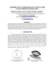
Ionospheric Ray-TracingEquations and their SolutionChristopher J. ColemanAbstractThe Haselgrove ray-tracing equations are deriveddirectly from Maxwell’s equations. Some methods for theirsolution are discussed. In particular, we look at reducedversions of the equations that allow fast numerical solutionand, in some cases, analytic solution.1. IntroductionIt is now over 50 years since Jenifer Haselgroveintroduced the ray-tracing equations that have becomesynonymous with her name. During this time, her equationshave become a major tool for investigating radiowavepropagation in the ionosphere. In the early days, suchstudies were needed because of the importance of ionosphericpropagation for long-range terrestrial communications. Suchcommunications take place at high frequencies (HF), anduse the fact that radiowaves at HF (3 to 30 MHz) arerefracted back down to the Earth by the ionosphere. However,with the advent of artificial satellites, ionosphericcommunication has become less important. Nevertheless,such communications are still an important tool for themilitary, aid agencies, and remote communities.Furthermore, the introduction of over-the-horizon radar(OTHR) has significantly increased the use of ionosphericpropagation. The extreme demands of over-the-horizonradar have made it necessary to understand ionosphericpropagation at a more refined level, and the Haselgroveequations have played an important part in such studies.Starting with the Haselgrove equations, we reviewsome of the ray-tracing approaches that are available for thestudy of ionospheric propagation. In Section 2, we derivethe Haselgrove equations directly from Maxwell’s equations(together with some basic plasma physics). Derivations ofthe Haselgrove equations tend to use ray optics, in particularthe Hamiltonian equations, as their starting point [1-3].Section 2 attempts to start from a more fundamental position,and to cast the equations as part of a procedure for thesolution of Maxwell’s equations in the high-frequencylimit. In [4], it was found that the Runge-Kutta-Fehlbergnumerical scheme constituted a very efficient means ofsolving the Haselgrove equations, and so we include a briefdescription of this algorithm. Unfortunately, there still existray-tracing applications for which computer solutions tothe Haselgrove equations are not fast enough. A particularcase is the coordinate registration (CR) problem of overthe-horizonradar. In the coordinate-registration problem,fast ray tracing is required to convert the radar range (thetime for the radio signal to travel to the target) into the actualground range. Due to the ever-changing nature of theionosphere, these calculations need to be done in real time.Consequently, in Sections 3 to 5 we look at somesimplifications to the Haselgrove equations that can providethis increased speed. In Section 3, we look at the situationwhere the background magnetic field can be regarded asbeing weak (a good approximation for most HF frequenciesabove 10 MHz). In Section 4, we look at the simplificationthat results when we totally ignore the background magneticfield, an approximation that can be made more respectableby the use of effective wave frequencies. Finally, in Section 5,we consider some first integrals of the ray-tracing equations,and we also consider analytic solutions that can be derivedfrom these first integrals.2. The Haselgrove EquationsFor time-harmonic fields in a vacuum, Maxwell’sequations yield the field equations20 0 0∇×∇× E− ω µ ε E = − jωµJ , (1)where E is the time-harmonic electric field, J is the timeharmoniccurrent density, and ω is the wave frequency.Within the ionospheric plasma, the motion of an electronsatisfiesChristopher J. Coleman is with the School of Electricaland Electronic Engineering, University of Adelaide,Adelaide, SA 5005, Australia;e-mail: ccoleman@eleceng.adelaide.edu.auTheRadio Science Bulletin No 325 (June 2008) 17
Page 4 and 5: URSI Forum on Radio Scienceand Tele
Page 6 and 7: URSI Accounts 2007Income in 2007 wa
Page 8 and 9: EURO EUROA2) Routine Meetings 5,372
Page 10 and 11: URSI Awards 2008The URSI Board of O
Page 12 and 13: • Compatibility refers to the abi
Page 14 and 15: Introduction to Special Sections Ho
Page 18 and 19: mwÆ = eE + ew× B −mνw , (2)whe
Page 20 and 21: Haselgrove equations [2]. Furthermo
Page 22 and 23: anddQ 1 r ∂n= + n −Qdθ2 2 2n
Page 24 and 25: Ray Tracing ofMagnetohydrodynamic W
Page 26 and 27: Figure 1a. The refractive-index sur
Page 28 and 29: 2 ⎡ ∂VAj, ∂VS⎤ω ⎢VAj, +
Page 30 and 31: ( ω kV j j)dx ∂i 0 + ∂ω0,= =
Page 32 and 33: compared with the wavelength, i.e.,
Page 34 and 35: decreasing to half their value in a
Page 36 and 37: Practical Applicationsof Haselgrove
Page 38 and 39: **.modeled TID ionospheres using Ha
Page 40 and 41: ∂ϕ∂ϕ1 kϕ∂r=− +, (12)∂
Page 42 and 43: screen (which is implemented in a s
Page 44 and 45: directed boresight and, similar to
Page 46 and 47: Typical OTH radar ionospheric sound
Page 48 and 49: ay-homing calculations for analyzin
Page 50 and 51: Figure 1. A Cartesian geometry cons
Page 52 and 53: orc dϕh′ = , (5a)4πdfincreases
Page 54 and 55: in four runs by five rays, giving a
Page 56 and 57: GPS : A Powerfull Tool forTime Tran
Page 58 and 59: altitude of ~26562 km will tick mor
Page 60 and 61: Each component of the errors is ass
Page 62 and 63: Figure 3. The effect of GPS timeerr
Page 64 and 65: Figure 6. The frequencystability of
Page 66 and 67:
Figure 9. The participating laborat
Page 68 and 69:
unlike the possibility of a gap in
Page 70 and 71:
Table 5. The capabilities of GPS ti
Page 72 and 73:
12. References1. C. Audoin and J. V
Page 74 and 75:
ConferencesCONFERENCE REPORT12TH IN
Page 76 and 77:
URSI CONFERENCE CALENDARURSI cannot
Page 78 and 79:
The Journal of Atmospheric and Sola
Page 80:
APPLICATION FOR AN URSI RADIOSCIENT
show all

Radio Science Bulletin 325 - June 2008 - URSI

You also want an ePaper? Increase the reach of your titles

Delete template?

Save as template?