Radio Science Bulletin 325 - June 2008 - URSI

More documents

Recommendations

Info

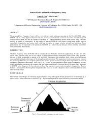
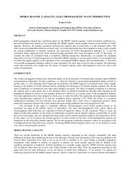
Figure 1a. The refractive-index surface formagnetohydrodynamic waves when the sound speedis less than the Alfvén speed.Figure 1b. The refractive-index surface formagnetohydrodynamic waves when the sound speedis greater than the Alfvén speed.points located a distance ± VAfrom the origin in thedirection of the magnetic field.Examples of ray surfaces for the magnetosonic wavesare shown in Figure 2. The surface for the fast wave in theupper panel is an ovoid, showing the magnitude of thegroup velocity (equivalent in this nondispersive case to theray velocity) as a function of direction. The surface for theslow wave is more complicated. It can be understood byconsidering Figure 1a, which shows the correspondingrefractive-index surface. For slow-wave propagation withthe wave normal parallel to the field in the positive direction,the ray direction normal to the surface is also parallel to thefield. As we increase the angle between the wave normaland the magnetic field anticlockwise, the angle between theray direction and magnetic field increases clockwise, untilit reaches a maximum value where there is a point ofinflection in the refractive-index surface. At this point,there is a cusp in the ray surface. As the wave-normal angleincreases further, the ray direction again decreases. Bothray- and refractive-index surfaces are surfaces of rotationabout the magnetic-field direction.the plasma rest frame be ω 0 . The frequency in the observer’sframe is then Doppler shifted so thatω0= ω − k • V . (10)The dispersion relations are then those for a stationarymedium, Equations (2) and (4), with ω replaced byω − k•VIn MHD propagation, a point source radiates waveshaving the shape of the ray surface. The ray surface alsorepresents the shape of a pulse spreading out from thesource, since the medium is nondispersive and wavefrontsand signal fronts have the same shape. The ray surface is thecorrect surface to use in Huygens’ construction.2.2. Moving MediaIn uniform moving media, the situation is complicated.Suppose the plasma moves in the reference frame of theobserver with velocity V. Let the frequency of the wave inFigure 2. Ray surfaces for the fast and slow waves.26TheRadio Science Bulletin No 325 (June 2008)
In the moving medium, there is no longer a single axisof rotational symmetry. There are two characteristic axesparallel to the magnetic field and the flow velocity. Therefractive-index surfaces are now reflection symmetricacross the plane defined by B and V.The ray is still normal to the refractive-index surface.The group velocity isV G =∇ k ω( )=∇ k ω 0 + k•V (11)=∇ k ω 0 +V= VG,0+ V ,giving the fairly obvious result that the group velocity in themoving medium is the resultant of the group velocity in therest frame and the velocity of the medium. In the particularcase of the transverse Alfvén wave,VG= VA+ V , (12)and the group velocity in the moving medium is not parallelto B. For example, in observations of the solar wind bysatellites at the solar libration point, such as WIND or ACE,since V >> V A , transverse Alfvén waves are propagatedalmost radially from the sun, rather than parallel to themagnetic field.3. Theory of Ray Tracing3.1 Stationary MediaRay tracing applies when a medium is slowly varying.By this it is meant that the medium does not changeappreciably within a wavelength. The ray-tracing equationsin a stationary medium – as shown, for example, by Walker[2] – are given byd r =∇kω, (13)dtdk =−∇ω ,dtor in Cartesian tensor notation,dxidtdkidt∂ω= , (14)∂ ki∂ω=− ,∂ xwhere the subscripts take the values 1, 2, 3, correspondingto the three Cartesian coordinate directions, and summationon the repeated subscript is understood. Precise evaluationsof the errors depend on the specific circumstances of theproblem. Examples of such error calculations were givenby Walker [4, Section 15.4.2] for a particular case, forexample. Such calculations show that even when the mediumchanges by as much as 10% per wavelength, the error inphase is less than one radian in 200π wavelengths. Theaccuracy of the ray tracing depends on the precision withwhich the phase is known, and in most ray-tracing situations,the medium varies far more slowly than this.Let us first consider the trivial case of transverseAlfvén waves, and show that the ray-tracing equations do,in fact, give rays following the field lines with the Alfvénspeed. From Equation (1), with the choice of the positivesign, we getidrk( A)Adt =∇ k • V = V , (15)dk( A )dt =−∇ k • V .As expected, the first of these shows that the wave packetmoves parallel to V A , and hence to B. (The choice of theother sign would have given a wave packet moving antiparallelto B). The second equation shows how thewavenumber, and hence the wavelength, change along theray but are independent of the first equation. Thus, ratherthan two simultaneous vector differential equations for theray path, we can evaluate the change of ray path and thechange of wavelength independently. For the magnetosonicwaves, we evaluate the expressions on the right-hand sideof Equation (15) explicitly using Equation (4). The result,in Cartesian tensor notation, is( + ) ω − ( , )2 2 2 2ω⎡2ω− ( A + S )⎤⎡k V V k k V Vdx ⎢i=⎣dt⎢k V V⎣⎥⎦2 2 2 2 2i A S i j A j S( kV )2 2j A, j kVSVA,i2 2 2 2− , (16)ω ⎡ 2ω− k ( VA+ VS) ⎤⎢⎣⎥⎦⎤⎥⎦TheRadio Science Bulletin No 325 (June 2008) 27
Page 4 and 5: URSI Forum on Radio Scienceand Tele
Page 6 and 7: URSI Accounts 2007Income in 2007 wa
Page 8 and 9: EURO EUROA2) Routine Meetings 5,372
Page 10 and 11: URSI Awards 2008The URSI Board of O
Page 12 and 13: • Compatibility refers to the abi
Page 14 and 15: Introduction to Special Sections Ho
Page 16 and 17: In the December 2008 issue, Part 2
Page 18 and 19: mwÆ = eE + ew× B −mνw , (2)whe
Page 20 and 21: Haselgrove equations [2]. Furthermo
Page 22 and 23: anddQ 1 r ∂n= + n −Qdθ2 2 2n
Page 24 and 25: Ray Tracing ofMagnetohydrodynamic W
Page 28 and 29: 2 ⎡ ∂VAj, ∂VS⎤ω ⎢VAj, +
Page 30 and 31: ( ω kV j j)dx ∂i 0 + ∂ω0,= =
Page 32 and 33: compared with the wavelength, i.e.,
Page 34 and 35: decreasing to half their value in a
Page 36 and 37: Practical Applicationsof Haselgrove
Page 38 and 39: **.modeled TID ionospheres using Ha
Page 40 and 41: ∂ϕ∂ϕ1 kϕ∂r=− +, (12)∂
Page 42 and 43: screen (which is implemented in a s
Page 44 and 45: directed boresight and, similar to
Page 46 and 47: Typical OTH radar ionospheric sound
Page 48 and 49: ay-homing calculations for analyzin
Page 50 and 51: Figure 1. A Cartesian geometry cons
Page 52 and 53: orc dϕh′ = , (5a)4πdfincreases
Page 54 and 55: in four runs by five rays, giving a
Page 56 and 57: GPS : A Powerfull Tool forTime Tran
Page 58 and 59: altitude of ~26562 km will tick mor
Page 60 and 61: Each component of the errors is ass
Page 62 and 63: Figure 3. The effect of GPS timeerr
Page 64 and 65: Figure 6. The frequencystability of
Page 66 and 67: Figure 9. The participating laborat
Page 68 and 69: unlike the possibility of a gap in
Page 70 and 71: Table 5. The capabilities of GPS ti
Page 72 and 73: 12. References1. C. Audoin and J. V
Page 74 and 75: ConferencesCONFERENCE REPORT12TH IN
Page 76 and 77:
URSI CONFERENCE CALENDARURSI cannot
Page 78 and 79:
The Journal of Atmospheric and Sola
Page 80:
APPLICATION FOR AN URSI RADIOSCIENT
show all

Radio Science Bulletin 325 - June 2008 - URSI

Create successful ePaper yourself

Delete template?

Save as template?