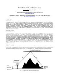
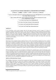
decreasing to half their value in a time such that T = 1000 s.This was a much larger change than would be typical of thereal magnetotail, but illustrated the physics of the problem.1The initial frequency used in the computation was 0.5 s − .However, since all frequencies have the same group andphase velocity, the ray paths calculated were independentof ω , and the change in frequency was proportional to theinitial frequency. Thus, the results applied to any frequency,provided that it was not so low that the slowly-varyingcriterion was violated.The results are shown in Figure 5 for a wave packetthat started at 22.5R E from the current sheet. Figure 5ashows the ray path, and Figure 5b shows the change in thefrequency ω . Ticks are shown along the ray pathrepresenting equal intervals of time. As the medium wascompressed, the magnitudes of the magnetic field and thedensity were doubled, and the Alfvén speed increased by afactor of 2. Since the wavelength was unchanged, thefrequency f = V λ was increased by the same factor.AIn interpreting this diagram, it is important tounderstand that there are significant differences from thebehavior shown in a stationary or a steady-state medium. Ifthere is no dependence on t, successive parts of a wave of agiven frequency follow the same path. The ray path isindependent of time. When the medium varies in time, partsof the wave passing through a given point follow differentpaths as the medium changes. To clarify this, considerFigure 6. Imagine that at time t = 0 , just as the compressionis becoming appreciable, we have a continuous transverseAlfvén wave limited in space, forming a thin pencil alignedwith the magnetic field and represented by the line ABCD.Assume also that the wave normal is in the x direction. Thepoints A, B, C, and D are equally spaced and separated byan integral number of wavelengths. We consider the locationof the signal at a succession of times: t 1 , t 2 , etc., separatedby equal intervals. Each portion of the pencil moves alonga ray path like that of Figure 5a. Wave packets that initiallyfollowed each other along a single ray path parallel to thefield now follow different paths as the medium changes intime. At consecutive equal time intervals, the signal occupiesa pencil defined by the change in position of the wavepackets at A, B, C, and D. The horizontal distance betweenthese points remains constant, and thus the wavelengthcannot change. However, the velocity is increasing, as canbe seen from the fact that the horizontal distance betweensuccessive positions of each point increases. Thus, thefrequency must also increase. The net effect of thecompression is that the wave, initially confined to a fieldline and propagated along it, continues to be confined to thesame frozen-in field line as it is carried inwards by thecompression. As this happens, the velocity and frequencyincrease.This is an illuminating example that keeps clear thedistinction between temporal and spatial effects. In morecomplicated cases, spatial and temporal effects areinextricably interconnected.5. Discussion and ConclusionsRay tracing has not often been used as a technique foranalyzing the behavior of MHD waves in geospace.Frequently, the wavelengths are so large that the mediumcannot be regarded as slowly varying, so that full-wavetreatments are necessary. In addition, characteristic waveFigure 5. Ray tracing in amodel in which the magneticfield is increasing with time:−1V A ,0 = 0.01 REs,−1ω 0 = 0.5 s , T = 1000 s ,f = 1.0 . (a) The ray pathof a wave packet. (b) Thechange in frequency withmagnetic field increase as afunction of time.34The<strong>Radio</strong> <strong>Science</strong> <strong>Bulletin</strong> No <strong>325</strong> (<strong>June</strong> <strong>2008</strong>)
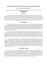
Figure 6. The motion of a ray pencil that is aligned with the magnetic field.velocities are small, so that the motion of the medium issignificant. The velocity of the medium relative to theobserver is sufficient to influence the dispersion relationsubstantially as a result of Doppler shift, whereas at radiofrequencies the wave velocities are usually large enough sothat the medium can be regarded as being at rest.In this paper, we have reviewed the ideas of raytracing for MHD waves in stationary media. We have thengeneralized them to apply to steady-state motion of themedium, in the same way as has been done for sound waves,for example, by Lighthill [3]. We have also presentedequations that allow for the tracing of rays in slowly varyingmedia with motion that is not steady-state flow. This is anew result, showing how the frequency may change alongthe ray as a result of Doppler shifts.It is not our intention in this paper to apply theequations to specific magnetospheric problems. However,it is worth considering the circumstances in which theywould be useful. One obvious case would be that of Pc3pulsations originating from the neighborhood of the bowshock. These are propagated from the shock through themagnetosheath, and are eventually transmitted into theionosphere. Ray-tracing studies of such waves in the past[5] have assumed a stationary medium. The magnetosheathhas strong streaming velocities past the magnetopause, butfor most purposes could be treated as being in a steady state.The steady-state equations would be appropriate, and thePc3 wavelengths are short enough for the ray-tracingapproximation to be valid. The examples in this papersuggest that this could lead to significant modifications ofthe results for a stationary medium.In the solar wind, the flow is supersonic and super-Alfvénic. It may in some regions approximate a steadystateflow, but usually this will not be the case. Theappropriate equations would be the general equations. Insuch a case, the model might often need to be so complicatedthat computation might not be worth while. Succeedingwave packets would not follow the same path as conditionschanged in time. Nevertheless, the equations make explicitthe fact that as each wave packet is propagated, its frequencychanges according to the third of Equations (31); attemptsto correlate spectral peaks observed at different locationsmay fail because of Doppler shifts.A topic that we have not discussed is the exchange ofenergy between background flows and the wave. In the caseof atmospheric winds, this can lead to modification of thebackground flow by the wave, and amplification orattenuation of the wave through the energy exchange. Studyof such processes in the solar wind is still to be carried out.It is hoped that these equations will be applied to thesolution of wave-propagation problems in geospace.6. References1. J. Haselgrove, “Ray Theory and a New Method for RayTracing,” in The Physics of the Ionosphere: Report of thePhysical Society Conference on the Physics of the Ionosphere,held at Cavendish Laboratory, Cambridge, September 1954,London, Physical Society, 1955, pp. 355-364.2. A. D. M. Walker, “Ray Tracing in the Magnetosphere,” <strong>Radio</strong><strong>Science</strong> <strong>Bulletin</strong>, No. 326, September <strong>2008</strong>, to appear.3. J. Lighthill, Waves in Fluids, Cambridge, Cambridge UniversityPress, 1978.4. A. D. M. Walker, Magnetohydrodynamic Waves in Geospace– The Theory of ULF Waves and their Interaction with EnergeticParticles in the Solar-Terrestrial Environment, Bristol,Institute of Physics Publishing, 2005.5. X. Zhang, R. H. Comfort, D. L. Gallagher, J. L. Green, Z. E.Musielak, and T. E. Moore, “Magnetospheric Filter Effect forPc3 Alfvén Mode Waves,” Journal of Geophysical Research– Space Physics, 100, 1995, pp 9585-9590.The<strong>Radio</strong> <strong>Science</strong> <strong>Bulletin</strong> No <strong>325</strong> (<strong>June</strong> <strong>2008</strong>) 35
- Page 4 and 5: URSI Forum on Radio Scienceand Tele
- Page 6 and 7: URSI Accounts 2007Income in 2007 wa
- Page 8 and 9: EURO EUROA2) Routine Meetings 5,372
- Page 10 and 11: URSI Awards 2008The URSI Board of O
- Page 12 and 13: • Compatibility refers to the abi
- Page 14 and 15: Introduction to Special Sections Ho
- Page 16 and 17: In the December 2008 issue, Part 2
- Page 18 and 19: mwÆ = eE + ew× B −mνw , (2)whe
- Page 20 and 21: Haselgrove equations [2]. Furthermo
- Page 22 and 23: anddQ 1 r ∂n= + n −Qdθ2 2 2n
- Page 24 and 25: Ray Tracing ofMagnetohydrodynamic W
- Page 26 and 27: Figure 1a. The refractive-index sur
- Page 28 and 29: 2 ⎡ ∂VAj, ∂VS⎤ω ⎢VAj, +
- Page 30 and 31: ( ω kV j j)dx ∂i 0 + ∂ω0,= =
- Page 32 and 33: compared with the wavelength, i.e.,
- Page 36 and 37: Practical Applicationsof Haselgrove
- Page 38 and 39: **.modeled TID ionospheres using Ha
- Page 40 and 41: ∂ϕ∂ϕ1 kϕ∂r=− +, (12)∂
- Page 42 and 43: screen (which is implemented in a s
- Page 44 and 45: directed boresight and, similar to
- Page 46 and 47: Typical OTH radar ionospheric sound
- Page 48 and 49: ay-homing calculations for analyzin
- Page 50 and 51: Figure 1. A Cartesian geometry cons
- Page 52 and 53: orc dϕh′ = , (5a)4πdfincreases
- Page 54 and 55: in four runs by five rays, giving a
- Page 56 and 57: GPS : A Powerfull Tool forTime Tran
- Page 58 and 59: altitude of ~26562 km will tick mor
- Page 60 and 61: Each component of the errors is ass
- Page 62 and 63: Figure 3. The effect of GPS timeerr
- Page 64 and 65: Figure 6. The frequencystability of
- Page 66 and 67: Figure 9. The participating laborat
- Page 68 and 69: unlike the possibility of a gap in
- Page 70 and 71: Table 5. The capabilities of GPS ti
- Page 72 and 73: 12. References1. C. Audoin and J. V
- Page 74 and 75: ConferencesCONFERENCE REPORT12TH IN
- Page 76 and 77: URSI CONFERENCE CALENDARURSI cannot
- Page 78 and 79: The Journal of Atmospheric and Sola
- Page 80: APPLICATION FOR AN URSI RADIOSCIENT