Radio Science Bulletin 325 - June 2008 - URSI

URSI Forum on Radio Scienceand TelecommunicationsApplications implemented through radiocommunication are exploding. This trend is likely toaccelerate and, accordingly, the operation of many passiveand active radio services will become dependent on thereliability of the new communication systems. All scientistsengaged in radio-science activities must be aware of potentialchallenges and novel developments, and should be in aposition to express their interest or/and concern. It is theobjective of the “Forum on Radio Science andTelecommunications,” organized on August 15 during the2008 URSI GA in Chicago, to provide information, and toencourage exchanges on all domains of radio science andtheir relation to telecommunications.The Forum will address the potential and challengesof novel developments in wireless telecommunications,which are of prime importance to anyone involved in radioscience and system development, both from a user’s and apolicy maker’s standpoint. It will have four invited papersof 40 minutes (25 minutes presentation plus 15 minutesdiscussion time) each, followed by a panel discussion. Thepapers will aim at stimulating discussions. The paneldiscussion of 40 minutes will focus on possible activities/actions for URSI to deploy in this area.The following subjects will be presented and discussed:1. “Cognitive Radio” by Hiroshi Harada (JP)Wireless systems in which the networks and/or the radiostations are sufficiently intelligent to provide and/or use(“grab”) radio resources flexibly and adaptively;2. “Ultra-wideband Wireless Systems” by Andy Molisch(USA)Systems employing ultra-large bandwidth and/or signalsof ultra-low spectral density; their unique features,potentials, and weaknesses;3. “Interference Management” by Lilian Jeanty (NL)Novel methods to protect communication and remotesensingsystem integrity and to regulate spectrum usagein a dynamic and flexible manner, while catering toultra-wideband and intelligent radio systems;4. Health aspects of the proliferation of wirelesscommunications in a deregulated arena by NielsKuster (CH).For the panel discussion, brief interventions (twominutes) may be prepared to complete the information or toraise specific points, such as:• Other new trends in radio-system development• Specific issues for the URSI Commissions• New radio-science research areas to be developed inrelation to new wireless services• Possible URSI contributions to international discussions,the development of standards and regulationsThe Forum discussions should result in the definitionof follow-up actions (e.g., by one or more URSI workinggroups) to establish a more permanent role for URSI inrepresenting the interests of radio science in worldwidediscussions on the development of wireless communications.Gert BrussaardRadicom ConsultantsHendrik van Herenthalslaan 115737 ED Lieshout, NetherlandsTel: +31 499 425430E-mail: gert.brussaard@radicom.nl4TheRadio Science Bulletin No 325 (June 2008)

Receiving the Radio ScienceBulletin for the Next TrienniumThe Radio Science Bulletin has historically been provided in print form by mail to all URSIRadioscientists. URSI Radioscientists are those who have registered for the most-recent past URSIGeneral Assembly (the registration fee includes 40€ as the mandatory fee for becoming an URSIRadioscientist for the triennium), or those who apply to the URSI Secretariat to become URSIRadioscientists (and pay the fee) between General Assemblies. The Bulletin has also been sent inprint form by mail to URSI Member Committees, and some libraries.The costs of printing and mailing the Bulletin have increased dramatically over the pasttriennium, and the Web has become a viable alternative method of disseminating publicationsmuch more rapidly than is possible using ordinary mail. The version of the Bulletin available viathe Web is also in color, in contrast to the printed version. In the interest of controlling costs andbeing able to continue to provide the Radio Science Bulletin to all URSI Radioscientists, at its Maymeeting the URSI Board decided to adopt a new policy for delivering the Bulletin in the comingtriennium. Beginning with the XXIXth General Assembly in Chicago, 40€ will continue to beincluded as a required part of the registration fee to become an URSI Radioscientist (this is theapproximate current cost of producing and publishing the Bulletin for the triennium, without thecost of printing and mailing individual copies). Starting with the March 2009 issue, all URSIRadioscientists will receive an e-mail alert when the Bulletin is available for download from theURSI Web site. If an URSI Radioscientist wishes to continue to receive a printed copy of theBulletin by mail, he or she may pay an additional optional fee of 60€ to cover the printing andmailing costs for the triennium. Printed copies of the Bulletin will continue to be sent to MemberCommittees and libraries.TheRadio Science Bulletin No 325 (June 2008) 5

URSI Accounts 2007Income in 2007 was higher than average due to the fact that somemember committees paid their arrears and some paid their dues inadvance. We also received the remainder of the fees of the GA2005from New Delhi. Total income from the 2005 GA was approx. EUR81,500 which is far less than the total cost of the GA to URSI which wasaround EUR 140,000. In real market value in EUR the investmentshave gained value even when taking into account the drop of the USD.The net total URSI assets have increased considerably. However, asignificant part of these assets are allocated. The allocations include animportant provision for the 2008 GA, leaving a reserve of less thanEUR 100,000.On the expenditure side the following points are noteworthy:· The cost of the Coordinating Committee meeting: EUR 18,929.09BALANCE SHEET: 31 DECEMBER 2007ASSETS EURO EURODollarsMerrill Lynch WCMA 574.20Fortis 1,310.50Smith Barney Shearson 5,509.55_________7,394.25EurosBanque Degroof2,483.33Fortis 52,939.57_________55,422.90InvestmentsDemeter Sicav Shares 22,681.79Rorento Units 111,414.88Aqua Sicav 63,785.56Merrill-Lynch Low Duration (304 units) 3,268.17Massachusetts Investor Fund 250,483.18Provision for (not realised) less value (7,472.37)Provision for (not realised) currency differences (80,263.20)_________363,898.01684 Rorento units on behalf of van der Pol Fund 12,414.34_________376,312.35Short Term Deposito 201,139.20Petty Cash 942.15__________Total Assets 641,210.85Less CreditorsIUCAF 10,778.95ISES 11,110.14_________(21,889.09)Balthasar van der Pol Medal Fund (12,414.34)NET TOTAL OF URSI ASSETS 606,907.426· The expenditure to the Commissions: EUR 33,897.50· The travel and representation costs of the Board: EUR 17,091.54The latter point reflects the increased efforts by the Board in representingURSI interests in international organisations. In the budget for the nexttriennium, therefore, a new item: “Travel by the Board” will be added.Also, provisions will be made for the Regional Centre in New Delhi.The Board is seriously considering means to limit the loss on futureGeneral Assemblies. There are three possibilities to accomplish this:reduce the travel cost of URSI officials, increase the revenue, or reducethe cost of the General Assembly by requiring less infrastructuraldemands for organizing it.The General Secretariat has handled the day-to-day finances in itsusual very efficient way, for which our sincere thanks.G. Brussaard,Treasurer, URSITheRadio Science Bulletin No 325 (June 2008)

The net URSI Assets are represented by: EURO EUROClosure of SecretariatProvision for Closure of Secretariat 90,000.00Scientific Activities FundScientific Activities in 2008 45,000.00Publications in 2008 40,000.00Young Scientists in 2008 40,000.00Administration Fund in 2008 85,000.00Scientific Paper submission software in 2008 30,000.00I.C.S.U. Dues in 2008 3,600.00_________243,600.00XXIX General Assembly 2008 Fund:During 2006-2007-2008 180,000.00_________Total allocated URSI Assets 513,600.00Unallocated Reserve Fund 93,307.42_________606,907.42Statement of Income and expenditure for the year ended 31 December 2007I. INCOME EURO EUROGrant from ICSU Fund and US NationalAcademy of Sciences 0.00Allocation from UNESCO to ISCU Grants Programme 0.00UNESCO Contracts 0.00Contributions from National Members (year -1) 33,578.29Contributions from National Members (year) 170,577.70Contributions from National Members (year +1) 38,789.50Contributions from Other Members 0.00Special Contributions 0.00Contracts 0.00Sales of Publications, Royalties 0.00Sales of scientific materials 0.00Bank Interest 3,534.04Other Income 46,173.50_________Total Income 292,653.03II. EXPENDITUREA1) Scientific Activities 54,026.74General Assembly 2005/2008 18,929.09Scientific meetings: symposia/colloqiua 33,897.50Working groups/Training courses 0.00Representation at scientific meetings 1,200.15Data Gather/Processing 0.00Research Projects 0.00Grants to Individuals/Organisations 0.00Other 0.00Loss covered by UNESCO Contracts 0.00TheRadio Science Bulletin No 325 (June 2008) 7

EURO EUROA2) Routine Meetings 5,372.04Bureau/Executive committee 5,372.04Other 0.00_________A3) Publications 34,266.58B) Other Activities 10,682.00Contribution to ICSU 4,682.00Contribution to other ICSU bodies 6,000.00Activities covered by UNESCO Contracts 0.00_________C) Administrative Expenses 74,350.69Salaries, Related Charges 61,956.64General Office Expenses 3,313.14Travel and representation 17,091.54Office Equipment 3,081.30Accountancy/Audit Fees 5,187.88Bank Charges/Taxes 2,555.02Loss on Investments (realised/unrealised) (18,834.83)_________Total Expenditure: 178,698.05Excess of Income over Expenditure 113,954.98Currency translation difference (USD => EURO) - Bank Accounts (786.88)Currency translation difference (USD => EURO) - Investments (18,461.57)Currency translation difference (USD => EURO) - others 0.00Accumulated Balance at 1 January 2007 512,200.89_________606,907.42Rates of exchange:January 1, 2007December 31, 2007$ 1 = 0.7590 EUR$ 1 = 0.6860 EUREUROBalthasar van der Pol Fund684 Rorento Shares: market value on December 31(Aquisition Value: USD 12.476,17/EUR 12.414,34) 29,815.56Market Value of investments on December 31, 2006/2005Demeter Sicav 60,201.90Rorento Units (1) 566,670.00Aqua-Sicav 85,579.79M-L Low Duration 2,070.84Massachusetts Investor Fund 163,944.94_________878,467.48(1) Including the 684 Rorento Shares of the van der Pol Fund8TheRadio Science Bulletin No 325 (June 2008)

I. INCOMEAPPENDIX: Detail of Income and ExpenditureEUROEUROOther IncomeIncome General Assembly 2002 0.00Income General Assembly 2005 46,173.50Revenu Taxes 0.00__________46,173.50II . EXPENDITUREGeneral Assembly 2005Organisation 0.00Vanderpol Medal 0.00Expenses officials 0.00Young scientists 0.00_________Symposia/Colloquia/Working Groups:Commission A 0.00Commission B 9,000.00Commission C 3,000.00Commission D 2,500.00Commission E 0.00Commission F 3,500.00Commission G 3,000.00Commission H 2,000.00Commission J 0.00Commission K 9,000.00Central Fund 1,897.50_________0.0033,897.50Contribution to other ICSU bodiesUNESCO-ICTP 0.00FAGS 4,000.00IUCAF 2,000.00_________6,000.00Publications:Printing ‘The Radio Science Bulletin’ 12,708.78Mailing ‘The Radio Science Bulletin’ 21,557.80URSI Leaflet 0.00_________34,266.58TheRadio Science Bulletin No 325 (June 2008) 9

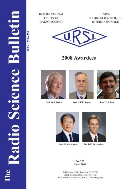
URSI Awards 2008The URSI Board of Officers decided at their May 2008 meeting in Ghent to follow the recommendations of the AwardsPanel and to give the 2008 Awards to the following distinguished scientists:The Balthasar Van der Pol Gold MedalThe Balthasar Van der Pol Gold Medal was awarded toProf. William J. Welch with te citation:“Pioneer of millimeterwavelenght interferometry toinvestigate astronomicalobjects ranging from solarsystem planets to galaxies atthe edge of the Universe withspectral and angularresolution”John Howard Dellinger Gold MedalThe John Howard Dellinger Gold Medal was be awarded toProf. Alan Ernest E. Rogers with te citation:“For his outstandingcontributions toinstrumentation in radioastronomy and its use tomake fundamentaldiscoveries aboutinterstellar masers,superluminal expansionof quasars, deuteriumabundance in the galaxy,and plate tectonics”Appleton PrizeAfter considering the views submitted by the AwardsAdvisory Panel, the Board of Officers submitted a short listof candidates in order of preference, with reasons for theorder, to the Royal Society.The Council of the Royal Society approved therecommendation of the URSI Board to award the 2008Appleton Prize to Prof. U.S. INAN with the citation:For fundamental contributionsto understandingof whistler-mode waveparticleinteraction in near-Earth space and the electrodynamiccoupling betweenlightning discharges andthe upper atmosphereBooker Gold MedalThe Booker Gold Medal was awarded to Prof. H. Matsumotowith te citation:Koga Gold Medal“For his outstandingcontributions to theunderstanding of nonlinearplasma waveprocesses, promotion ofcomputer simulations inspace plasma physicsand internationalleadership in plasmawave research”The Koga Gold Medal was awarded to Dr. D.F. Sievepiper,with te citation:The Awards were presented to theAwardees during the OpeningCeremony of the XXIXth GeneralAssembly in the Grand Ballroom ofthe Hyatt Regency Chicago Hotel,United States, on 10 August 2008“For contributions tothe development ofartificial impedancesurfaces and conformalantennas”10TheRadio Science Bulletin No 325 (June 2008)

URSI and the International Committeeon Global Navigation SatelliteSystems (ICG): An Update1. BackgroundSince its inaugural meeting in November 2006, URSIhas been participating in the International Committee onGlobal Navigation Satellite Systems (ICG) as an observer.I reported on the early activities in the Radio ScienceBulletin of March 2007.The following is a short summary of the background.The “Vienna Declaration on Space and HumanDevelopment” of the United Nations calls for universalaccess to and compatibility of space-based navigation andpositioning systems. In 2004, in Resolution 59/2, the UNGeneral Assembly invited the system and service providersto consider establishing an international committee onGNSS, in order to maximize the benefits of the use andapplication of GNSS to support sustainable development.The ICG was established and held its inaugural meeting inVienna in November 2006.The secretariat is provided by the UN Office for OuterSpace Affairs (OOSA) in Vienna. An Ad Hoc WorkingGroup meets twice yearly to discuss current issues, and toprepare the annual Plenary Meetings of the ICG.The ICG Terms of Reference define three types ofparticipants: Members, Associate Members, and Observers.Associate Members and Observers both may advise theCommittee and actively contribute to its work, but do nothave a vote. There is very little difference between AssociateMembers and Observers: the latter will not be called uponto contribute financially. Among others, COSPAR, theITU, and URSI participate as Observers. URSI’s interestsrange from the development of propagation models andsignal processing for radio navigation and positioning, tothe application of GNSS in radio-science research, andhence cover the work areas of several Commissions.At the first Plenary Meeting of the ICG in November2006, the work plan for the ICG was adopted. This plandefines four working groups:A. Compatibility and interoperabilityB. Enhancement of performance of GNSS servicesC. Information disseminationD. Interaction with national and regional authorities andrelevant international organizations, particularly indeveloping countriesThe Annex contains a summary of the work plan ofthe Working Groups.Furthermore, a Providers’ Forum (with exclusiveparticipation of providers of navigation satellite systems)was established, with the task to enhance compatibility andinteroperability among current and future systems.2. Second PlenaryMeetingof the ICG(Bangalore, September 5-7, 2007)2.1 Providers’ ForumImmediately preceding the second Plenary Meeting,a meeting of the Providers’ Forum was held on September4. The agenda included system and service updates fromeach of the following providers:• China: Compass/BeiDou Navigation Satellite System(CNSS)• India: Global Positioning System and Geostationary(GEO) Augmented Navigation System (GAGAN) andIndian Regional Navigation Satellite System (IRNSS)• Japan: Quasi-Zenith Satellite System (QZSS) andMultifunctional Transport Satellite (MTSAT) SatellitebasedAugmentation System (MSAS);• Russian Federation: Global Navigation Satellite System(GLONASS) and Wide-area System of DifferentialCorrections and Monitoring (SDCM);• United States: Global Positioning System (GPS) andWide-Area Augmentation System (WAAS);• European Community: European Satellite NavigationSystem (Galileo) and European GeostationaryNavigation Overlay Service (EGNOS).Key issues discussed included spectrum protection,compatibility and interoperability, orbital debris deconfliction,availability of a free and open service, timelyinformation dissemination, etc.All system providers agreed that as a minimum, allGNSS signals and services must be compatible. To themaximum extent possible, open signals and services shouldalso be interoperable. In this context, the following generaldefinitions were agreed upon:TheRadio Science Bulletin No 325 (June 2008) 11

• Compatibility refers to the ability of space-basedpositioning, navigation, and timing services to be usedseparately or together without interfering with eachindividual service or signal;• Interoperability refers to the ability of open global andregional satellite navigation and timing services to beused together to provide better capabilities at the userlevel than would be achieved by relying solely on oneservice or signal.2.2 Experts MeetingOn September 5, an Experts Meeting was held,consisting of five scientific and technical sessions:• Prediction of natural disaster and research on climatechange and Earth science• Geodetic reference frames• Atomic time standards, Coordinated Universal Time(UTC), and time transfer• Ionospheric/tropospheric models and space-weathereffects• GNSS activities in India2.3 Second Plenary MeetingThe second Plenary Meeting was held on September6 and 7. Reports from the Providers Forum and the WorkingGroups were presented, and the Committee considered therecommendations and plans for future work of the WorkingGroups. A special report was discussed on the subject ofSatellite-based Augmentation System certification.The Committee agreed that China be recognized as aprovider of GNSS, since it was developing the CompassNavigation Satellite System.Since this was only the second full meeting of theICG, several actions were proposed to streamline the workingmethods of the Working Groups and to avoid duplications.The Committee expressed its satisfaction with thecontinuing effort by the secretariat to develop the informationportal of the Committee as part of the Web site of the Officefor Outer Space Affairs.The Committee accepted the invitation of the UnitedStates to host the third meeting, to be held in 2008, andnoted the offer of the Russian Federation to host the fourthmeeting in 2009.Two informal meetings of the Ad Hoc WorkingGroup to prepare the next meeting of the Committee wereplanned for 2008.3. ConclusionsAll presentations from the Providers’ Forum and thetechnical expert sessions as well as the Working GroupReports are available at the portal of the Committee:http://www.unoosa.org/oosa/en/SAP/gnss/icg.htmlAfter a slow start, the work by the different WorkingGroups now seems to be developing. From the subjects ofthe technical sessions mentioned above, one can concludethat there are several areas where URSI is able to makecontributions. It is planned to prepare a report for the nextPlenary meeting, summarizing URSI’s interest in variousactivities. These include both research and developmentconcerning GNSS itself, and scientific applications of theuse of the positioning and navigation system. Inputs to thisreport will be solicited from the Commissions involved.4. Annex4.1 Summary of the ICG WorkPlan and Working Group ActionsThe ICG work plan is executed by five WorkingGroups, which have defined a number of specific Actions.4.1.1 Working Group A:Compatibility and InteroperabilityThe working group formed to address compatibilityand interoperability, to be co-led by the United States ofAmerica and the Russian Federation, will pursue thefollowing actions:- Action A1: Establish a providers forum to enhancecompatibility and interoperability among current andfuture global and regional space-based systems.- Action A2: Organize a workshop(s) on measures beingtaken by Members, Associate Members, and Observersto enhance interoperability and compatibility of (1)global and regional space-based systems and (2) regionalground-based DGNSS.- Action A3: Survey the level of interoperability andstandardization among GNSS constellations andaugmentations in order to identify concrete steps thatcan be taken at different levels (regulatory, systemimplementation, user algorithms) to improveinteroperability and standardization. It is expected thatthe situation is well advanced in civil aviation andmaritime areas, the effort would therefore probablyneed to concentrate on land-based applications andusers.- Action A4: Consider guidelines for the broadcast ofnatural disaster alarms via GNSS.12TheRadio Science Bulletin No 325 (June 2008)

- Action A5: Develop a strategy for support by theInternational Committee of mechanisms to detect andmitigate sources of electromagnetic interference, takingexisting regulatory mechanisms into consideration.4.1.2 Working Group B:Enhancement of Performance ofGNSS ServicesAs a unique combination of GNSS service providersand major user groups, the Committee will work to promoteand coordinate activities aimed at enhancing GNSSperformance, recommending system enhancements, andmeeting future user needs. Specifically, the following actionswill be taken by a working group co-led by India and theEuropean Space Agency:- Action B1: Develop a reference document on modelsand algorithms for ionospheric and troposphericcorrections.- Action B2: Examine the problem of multipath andrelated mitigation actions affecting both GNSS systemsand user receivers, especially for mobile receivers.- Action B3: Examine the extension of GNSS service toindoor applications.4.1.3 Working Group C:Information DisseminationThe Committee will consider the establishment ofuser information centers by GNSS providers. Themaintenance of a globally focused Web site will be a majortask of these centers. The United Nations, through theOffice for Outer Space Affairs of the Secretariat and onbehalf of the Committee, will combine all the Web sites intoa single site to act as a portal for users of GNSS services.Therefore, the Office for Outer Space Affairs will lead aworking group to accomplish the following actions:- Action C1: Establish the International Committeeinformation portal, drawing on contributions fromMembers, Associate Members, and Observers of theCommittee. This will include a calendar of GNSSrelatedevents.- Action C2: Identify undergraduate and graduate courseson GNSS to be included on the Committee portal.- Action C3: Consider the possibility of disseminating alist of relevant textbooks on GNSS in English and otherlanguages through the Committee portal. Considerationwill also be given to developing a glossary of terms anddefinitions.- Action C4: Consider the use of the Regional Centres forSpace Science and Technology Education, affiliated tothe United Nations, to promote GNSS use andapplications.- Action C5: Identify international conferences whereMembers, Associate Members, and Observers will makepresentations on the existence and work of theInternational Committee. A list of such events will bemaintained on the Committee information portal.- Action C6: Develop a proposal for further mechanismsto promote the applications of GNSS.4.1.4 Working Group D:Interaction with National andRegional Authorities and RelevantInternational OrganizationsThe Committee will establish links with national andregional authorities and relevant international organizations,particularly in developing countries. The Committee willorganize and sponsor regional workshops and other typesof activity in order to fulfill its objectives. The FédérationInternationale des Géomètres (FIG), the InternationalAssociation of Geodesy (IAG), and the International GNSSService will co-lead the activities listed below:- Action D1: Define minimum operational performancestandards for GNSS performance monitoring networks.- Action D2: Establish a working group focused on sitequality, integrity, and interference monitoring (SQII).- Action D3: Establish a working group to develop astrategy for support by the International Committee ofregional reference systems (e.g., the African GeodeticReference Framework (AFREF), the European PositionDetermination System (EUPOS), the IAG ReferenceFrame Sub-Commission for Europe (EUREF), and theGeocentric Reference System for the Americas(SIRGAS)).- Action D4: Establish a working group to develop astrategy for support by the International Committee ofmechanisms to detect and mitigate sources ofelectromagnetic interference, taking existing regulatorymechanisms into consideration.4.1.5 Working Group E:CoordinationIn the future, the Committee will consider, makerecommendations, and agree on actions to promoteappropriate coordination across GNSS programs.Furthermore, the Committee will encourage its Members,Associate Members, and Observers to maintaincommunication, as appropriate, with other groups andorganizations involved in GNSS activities and applications,through the relevant channels within their respectivegovernments and organizations. The Committee could alsosupport the establishment of national and/or regionalplanning groups for GNSS that would address regulationsassociated with the use of GNSS services, and suggestorganizational models to use at the national level for cocoordinatingand governing GNSS use.Gert BrussaardRadicom ConsultantsHendrik van Herenthalslaan 115737 ED Lieshout, NetherlandsTel: +31 499 425430E-mail: gert.brussaard@radicom.nlTheRadio Science Bulletin No 325 (June 2008) 13

Introduction to Special Sections HonoringJenifer HaselgroveEven a significant historical achievement maydiminish in its apparent magnitude if too casually viewedthrough the prism of our present state. This is vividlyportrayed in the world of computing, where an informationage now looks back on enormous machines, with theirclumsy human interfaces and relatively small processingand memory capabilities. Of course, more careful scrutinyreveals that what was achieved with those relatively primitivecomputers was far from trivial. After all, the birth ofcomputers was concurrent with the second World War, andsuccess and failure could beseen in very stark terms.The first automatedcomputers emerged inGermany, the US, and theUK in the 1940s. EDSAC,the first UK generalpurposestored-programcomputer, wascommissioned atCambridge in 1949.In 1950s’ Cambridge,the scene was set for a youngPhD student named JeniferHaselgrove (Figure 1) tomake a remarkableconnection, which wouldend up greatly benefitingthe world’s radio-sciencecommunity.called orders, which may have been a bit confusing atfirst, but nothing like the terrible mistake made inFORTRAN and later languages, where instructions arecalled “statements.” Of course, programs didn’t all donumerical work – take the initial orders for example –and there had to be programs right from the beginningto read users’ programs and data and to print results.Those were part of a whole “library” of subroutines forstandard jobs, including numerical ones such ascalculating square roots, and even division, which wasn’toriginally built in. At first theoutput was directly on to ateleprinter, typing on paperat, I think, 7 characters asecond, but later that waschanged to punched tape likethe input, to be printed lateror while the machine got onwith the calculating. Theactual computing buildingwas the original AnatomyDepartment, and there was acoffin lift (elevator) in onecorner. I don’t think any of usbothered about that, though,even working alone in thebuilding in the middle of thenight. We all had to do someof that – machine time wasrare and valuable!According toFigure 1. Jenifer HaselgroveHaselgrove, “these wereheady days, where everything you did on a computer wasnew.” An abstract from her recent musings on those timesprovides insight, and it is curious to get a glimpse of theearly utilization of computer-science constructs that havestood the test of time, such as functions and libraries:The programming language was a simple mnemoniccode, for example, “A 150” meant “add the number instorage location 150 into the accumulator [the placewhere the current working number was].” You didn’thave to think in binary arithmetic, contrary to what youread in some historical accounts of early computersnowadays. The program (that spelling was settled on foruse even in Britain fairly early, after some argument)was typed on to 5-hole (teleprinter) paper tape and readinto the machine by a single built-in program of “initialorders.” The instructions making up programs wereJenifer Haselgrove hadbegun her tertiary educationafter moving to Cambridge (Figure 2) in 1948, where shestarted reading math. At that time, she connected with BrianHaselgrove when they both joined a music group, whichlistened to “long playing records,” a recording and playbacktechnology that intrigued them both. They married in 1951.In the same year, she moved to physics and the CavendishLaboratory. When meeting the seniors on the board of theCavendish Laboratory, Haselgrove was a little taken backto find them expressing relief that she was not interested inpractical or field work. Curious on whether she was runningup against some Cavendish misogyny, she was amused tohear later, after some discrete inquiry with the departmentalsecretary, that the panel was greatly concerned about thelack of “facilities” at the field station! Furthermore, thesecretary had chided the board for being silly, suggesting“they could use one bush and Haselgrove another.”14TheRadio Science Bulletin No 325 (June 2008)

Figure 2. Richard Haselgrove, Jenifer Haselgrove’s brother, supplied this photograph from earlierCambridge days. Jenifer is fourth from right, front row. Brian Haselgrove (her first husband) is fifthfrom right, front row. John Leech (her second husband) is fifth from left, back row.Haselgrove was just starting her research when shefell pregnant, and 1952/3 was spent preparing for andrearing her son. Her early postgraduate research wasperformed under the renowned radio scientist KennethBudden, where she started on radio propagation, spendingtime calculating the trajectory of short ray paths by hand.Many other researchers were similarly developingmathematical and analytic techniques and constructs tofurther the domain of radio ray tracing through that time.Shortly afterwards, in discussions with her husband –himself a highly respected mathematician who was nowworking with EDSAC in the math department – she wasencouraged to look at ways to solve the ray-propagationproblem on a computer. Her first work on the topic waspublished shortly afterwards, and over the next five years aseries of papers were published (all referenced in thearticles to follow). Subsequent to her breakthroughs, thereis record of numerous efforts in computer-based ray tracingemerging throughout the world. Jenifer Haselgrove haddeveloped the connection that resulted in the birth of hersecond creation, computer-based radio ray tracing. By theearly 1960s, the radio-science community was on board andwas enamored with her latest “child.” Through popular use,her name is now enshrined with the original formulations,viz., the Haselgrove Equations. The equations derive fromthe physical-principle formulations of William RowanHamilton and James Clerk Maxwell, when applied to radiopropagation in the ionosphere. Haselgrove herself referredto them as Hamilton’s ray equations.Haselgrove worked on ray-tracing problems incollaboration with her husband, until he died in 1964. Afterthat, she remarried to John Leech, another Cambridgemathematician who had worked and socialized with theHaselgroves through their careers. Jenifer Haselgroveworked as a computer scientist at Glasgow University, andretired in 1981.A two-part collection of articles in the June andDecember editions of the Radio Science Bulletin has beendeveloped. It amounts to a dedicated effort by a group ofradio scientists who have benefited from the path pioneeredby Jenifer Haselgrove, and have taken the time to honor thatachievement.Of note is the variety of applications to which theHaselgrove Equations and computer-based ray tracing havebeen applied. Topics include EHF, VLF, and HFelectromagnetic propagation in the magnetosphere;whistlers; HF communications; inter-satellitecommunications; HF radar; HF radio direction finding; andremote-sensing investigations of the ionosphere andmagnetosphere. Many of these topics are touched on withthe following papers. The same equations also providesolutions for acoustic ray tracing.Part 1 of the testimonial editions appears in this issue.It starts with a theoretical treatise by Coleman, whodemonstrates a method of deriving the Haselgrove Equationsdirectly from Maxwell’s equations. This is followed byanother theoretical developmental piece by Walker, whodemonstrates a derivation based on Fermat’s principle.Walker goes on to show some historical applications ofHaselgrove’s methods in modeling electromagneticpropagation in the magnetosphere.Nickich discusses his career and the foundational rolethat radio ray tracing, based on the Haselgrove Equations,played in this. Finally, Barnes discusses two applications ofray tracing at HF, pertaining to sounders and radar.TheRadio Science Bulletin No 325 (June 2008) 15

In the December 2008 issue, Part 2 of the testimonialeditions will appear. This will begin with a summary ofmultiple applications of the Haselgrove Equations by James.It will be followed by a historical summary of ray-tracingdevelopment by Bennett. Dyson discusses the impact of theHaselgrove Equations and ray tracing on his career in radioscience.Kimaru discusses a career that began almostsimultaneously with Haselgrove’s, which involved theapplication of her ray-tracing techniques to whistler andother wave propagation in the magnetosphere. The editionis completed with a compilation of applications by Bertel.Please enjoy this tribute to Jenifer Haselgrove and herachievements. In collating and researching for this work,we have been inspired by many of the great minds that havebrought us so far in radio science, but none more thanJenifer Haselgrove and those around her at Cambridge,which led to her famous formulation and her use of one ofmankind’s first computers to solve it. Our hope is that theseeditions draw your attention to those “heady days,” a personwho lived through them, and her achievements. Just asimportantly, it is hoped that it inspires you in your radioscienceendeavors so that someone may write about themwith great respect in the near future.Rod Barnes and Phil WilkinsonCo-Guest Editors,Special Sections Honoring Jenifer HaselgroveE-mail: rbarnes@rri-usa.org, phil@ips.gov.au16TheRadio Science Bulletin No 325 (June 2008)

Ionospheric Ray-TracingEquations and their SolutionChristopher J. ColemanAbstractThe Haselgrove ray-tracing equations are deriveddirectly from Maxwell’s equations. Some methods for theirsolution are discussed. In particular, we look at reducedversions of the equations that allow fast numerical solutionand, in some cases, analytic solution.1. IntroductionIt is now over 50 years since Jenifer Haselgroveintroduced the ray-tracing equations that have becomesynonymous with her name. During this time, her equationshave become a major tool for investigating radiowavepropagation in the ionosphere. In the early days, suchstudies were needed because of the importance of ionosphericpropagation for long-range terrestrial communications. Suchcommunications take place at high frequencies (HF), anduse the fact that radiowaves at HF (3 to 30 MHz) arerefracted back down to the Earth by the ionosphere. However,with the advent of artificial satellites, ionosphericcommunication has become less important. Nevertheless,such communications are still an important tool for themilitary, aid agencies, and remote communities.Furthermore, the introduction of over-the-horizon radar(OTHR) has significantly increased the use of ionosphericpropagation. The extreme demands of over-the-horizonradar have made it necessary to understand ionosphericpropagation at a more refined level, and the Haselgroveequations have played an important part in such studies.Starting with the Haselgrove equations, we reviewsome of the ray-tracing approaches that are available for thestudy of ionospheric propagation. In Section 2, we derivethe Haselgrove equations directly from Maxwell’s equations(together with some basic plasma physics). Derivations ofthe Haselgrove equations tend to use ray optics, in particularthe Hamiltonian equations, as their starting point [1-3].Section 2 attempts to start from a more fundamental position,and to cast the equations as part of a procedure for thesolution of Maxwell’s equations in the high-frequencylimit. In [4], it was found that the Runge-Kutta-Fehlbergnumerical scheme constituted a very efficient means ofsolving the Haselgrove equations, and so we include a briefdescription of this algorithm. Unfortunately, there still existray-tracing applications for which computer solutions tothe Haselgrove equations are not fast enough. A particularcase is the coordinate registration (CR) problem of overthe-horizonradar. In the coordinate-registration problem,fast ray tracing is required to convert the radar range (thetime for the radio signal to travel to the target) into the actualground range. Due to the ever-changing nature of theionosphere, these calculations need to be done in real time.Consequently, in Sections 3 to 5 we look at somesimplifications to the Haselgrove equations that can providethis increased speed. In Section 3, we look at the situationwhere the background magnetic field can be regarded asbeing weak (a good approximation for most HF frequenciesabove 10 MHz). In Section 4, we look at the simplificationthat results when we totally ignore the background magneticfield, an approximation that can be made more respectableby the use of effective wave frequencies. Finally, in Section 5,we consider some first integrals of the ray-tracing equations,and we also consider analytic solutions that can be derivedfrom these first integrals.2. The Haselgrove EquationsFor time-harmonic fields in a vacuum, Maxwell’sequations yield the field equations20 0 0∇×∇× E− ω µ ε E = − jωµJ , (1)where E is the time-harmonic electric field, J is the timeharmoniccurrent density, and ω is the wave frequency.Within the ionospheric plasma, the motion of an electronsatisfiesChristopher J. Coleman is with the School of Electricaland Electronic Engineering, University of Adelaide,Adelaide, SA 5005, Australia;e-mail: ccoleman@eleceng.adelaide.edu.auTheRadio Science Bulletin No 325 (June 2008) 17

mwÆ = eE + ew× B −mνw , (2)where m is the electron mass, e is the electron charge, νis the plasma collision frequency, w is the electron velocity,and B 0 is the magnetic field of the Earth. The plasmacurrent is given by eN w , where N is the electron density,Thus, for a time-harmonic field, Equation (2) reduces to00− jωεXE = UJ + jY× J , (3)2 2where U = 1− jν ω , X = ωpω , Y =− eB0mω , and2ωp = Ne ε0mis the plasma frequency. In the highfrequencylimit (ω →∞), we normally assume an electricfield of the form E = E 0 exp ( − jβϕ ) , where E 0 and ϕare both slowly varying functions of position andβ = ω µ 0ε0(see [5] and [6] for more informationconcerning the high-frequency approximation). Noting that( )2∇×∇× E =∇ ∇• E −∇ E ,and substituting the assumed form of solution intoEquation (1), we find the leading order in ω yields− jωµ0−∇ϕ( ∇ ϕ• E0) + ( ∇ ϕ• ∇ϕ) E0 − E0 = J (4)2 0βwhere J = J 0 exp ( − jβϕ ). From Equation (3), it followsthat− jωεXE = UJ + jY× J . (5)0 0 0 0The dot product of Equation (4) with∇ ϕ yieldsjωµ0∇ ϕ• E0 = ∇ ϕ• J . (6)2 0βEliminating ∇ ϕ • E0from Equation (4) using Equation (6),we obtain− jωµ∇ •∇ − 0 =2 0 −∇ ∇ • (7)0β0( ϕ ϕ 1) E ( J ϕ ϕ J )Eliminating E 0 using Equation (5),( ∇ ϕ•∇ϕ − 1)( UJ + jY× J ) = −X( J −∇ϕ∇ ϕ•J )0 0 0 0From the dot product of Equation (8) with ∇ ϕ , we obtain( ) ( ) ( )(8)−j∇ ϕ• Y× J0 = −j ∇ ϕ× Y • J0 = U − X ∇ ϕ•J0(9)Using this to eliminate ∇ ϕ • J0from Equation (8),( U∇ ϕ•∇ϕ− U + X) J 0− jX= ∇ ( Y) J0 jY J0( 1)U X ϕ ∇ ϕ × • − × ∇ ϕ •∇ ϕ −−(10)Without loss of generality, we choose Y1= Y andY2 = Y3 = 0 (i.e., the x 1 coordinate direction is in thedirection of the magnetic field). In this case, Equation (10)can be rewritten as2( )⎡ Up + X −U jYPp1p 3 −jYPp1p⎤2⎢⎥⎢2 2 2 ⎥⎢ 0 ( Up + X − U ) + jYPp2p3 −jYPp2 − jY ( p − 1)⎥J0 = 0⎢⎥2 2 2⎢ 0 jYPp3 + jY ( p − 1) ( Up + X −U ) − jYPp3p2⎥⎣⎦2(11)where p =∇ ϕ , p p p P = X U − X . Thiswill only have a nontrivial solution if the determinant of thematrix is zero, that is,= • , and ( )⎡( ) ( ) 2⎢2 + − 2 + − +2 2 3 2 22Up X U Up X U Y P p p⎣( 3 )( 2 )− + − 1 + − 1 = 0 , (12)⎥⎦2 2 2 2 2Y Pp p Pp p ⎤2from which either Up + X − U = 0 (in which case, E 0 isparallel to Y ), or2 2 2( Up + X −U ) −Y ( p −1)2 2( )( )2 2 2 21−Y P p −1 p − p = 0 , (13)for which E 0 has no component in the direction of Y .Returning to a general system of coordinates (NB:2Yp1= Y• p and Y = Y • Y ), we obtain from Equation (13)that2 2 2( Up + X −U ) −Y ( p −1)2 22 ⎡ 2 2( ) ( ) 2−P p −1 Y p p Y⎤⎢− •⎥= 0 . (14)⎣⎦Equation (14) is a first-order partial differential equationfor the phase field, ϕ , and this can be solved by standardmethods for partial differential equations. For the equation18TheRadio Science Bulletin No 325 (June 2008)

F( x, p ) = 0 , we can define a solution in terms ofcharacteristic curves (our rays). These, together with thevalues of ϕ along them, will satisfy the generalized Charpitequations (see [7], for example):dxdti( )4 pi=− 1 −X −Y ( p − 1 + X) −2pYX2 2 i2dxidϕdpi= = . (15)∂F ∂p 3i−∂F ∂xip ∂F ∂p∑j=1jThe above equations can be used to find the ray curvesin terms of the values of the phase factor, ϕ , along them.We will consider the collision-free case ( U = 1 ).Equation (14) then implies2( 1) ( 1 ) 2( 1)2 2 2 2 2p − −Y − PY + p − X + X2 2 2( ) ( )( ) 2−P p − 1 Y + P p − 1 Y• p = 0 . (16)Multiplying through by 1−X , Equation (16) can be recastF x, p = 0 , whereas ( )2( , ) = ( 2 −1) ( 1− −2)F x p p X Y( 1) ⎡2 ( 1 )2 2+ p − X − X − XY⎣j⎤⎦2 2( ) i( )− 2p p• Y −2Y p − 1 p• Y . (19)iIf we now introduce the new dependent variable2q = p − 1 X (as defined in [3]), we obtain( )( )dxi=−4pi1 −X − Y ( q + 1) −2pYdt2 2 2i2 2( ) i( )− 2p p• Y −2Y p − 1 p• Y , (20)iwhich is the Haselgrove equation for the advancement of p[2]. The other equation implied by Equation (15) requiresthe coordinated derivatives of F , that is2( p ) 2∂F ⎛∂X ∂Y⎞=− − 1 ⎜ + 2Y•⎟∂xi ⎝∂xi ∂xi⎠2 ⎡∂X2( ) ⎢ ( )∂Y⎤+ p −1 2−4X −Y − 2XY•⎥⎣∂xi∂xi⎦Consequently,( 1 ) ( 1)( ) 22 2+ X − X + X p − Y• p . (17)∂X∂X+ X − X + p − Y•p∂x∂xi2( 2 3 ) ( 1)( ) 2i∂F∂pi( )( )⎡i ( )2 2 2= 4pi1− X −Y p − 1 + 2p 2X 1− X − XY⎣⎤⎦i2( )( )∂Y+ 2p• X p − 1 Y•p . (21)∂xIntroducing the same dependent and independent variablesas for Equation (20), we obtain from Equation (15) that2 2( ) i ( )+ 2pX p• Y + 2YX p − 1 p• Y . (18)idp idt( 1) ( ) 22( 1 2 )2 2=⎧⎡p p Y X Y⎤⎨ ⎢− − + • + − − ⎥q⎩⎣ ⎦We introduce a new parameter, t , along thecharacteristic curves defined bydt =−Xdϕp ∂F ∂p3∑j=1and then Equation (15), together with a rearranged versionof Equation (18), yieldsjjj=1⎫ ∂X+ 2−3X⎬⎭ ∂ xi2( 1) ⎡2( ) j 2( 1)3∂Yj+ ∑ p − p• Y p − q+Y ⎤⎣j⎦ ∂ x(22)Equations (20) and (22) together constitute the originaliTheRadio Science Bulletin No 325 (June 2008) 19

Haselgrove equations [2]. Furthermore, recastingEquation (16) in terms of q [2], we obtain⎡ 2( ) ( ) ( )2 2 2q 1− X − Y + q Y p 2 1 X Y⎤⎢• + − −⎥+ 1− X = 0⎣⎦(23)from which q can be derived (note that there are twopossible values of q, corresponding to two of the possiblesolutions to Equation (11)). The corresponding current,and hence the electric field through Equation (5), can beobtained from the homogeneous Equations (11) using thecalculated values of p on the ray. However, Equations (11)do not determine the magnitude of the field. This must becalculated by tracking the power out from the source. Thiscan be done by tracing out ray tubes, and noting that within20 2 0Ap E η , must remainconstant (A is the cross-sectional area of the tube). Themagnitude of the electric field can then be calculated fromthe power.these tubes, the power, ( )There remains the issue of solving the above raytracingequations. Starting with some initial value, w () 0 ,for w , the system of ordinary differential equations,dw dt = W( w), can be solved using Runge-Kuttatechniques. This was suggested in the Haselgrove andHaselgrove paper [2]. If we start a ray at the Earth’s surface,the initial values of p are given by the direction cosines atthis starting point. However, the extreme variations that canexist in the ionosphere often make it necessary to vary theincrement in t at each stage of the solution process, in orderto maintain accuracy. Haselgrove and Haselgrove [2]suggested the introduction of a scaling to produce thiseffect, but the Runge-Kutta-Fehlberg (RKF) method (see[8] for example) can also achieve this.Consider the solution at time t and prospectiveincrement ∆ t . Form the vectors k1, k2, k3, k4, k5, andk through the process6k1( )=∆ tW w , (24)( )k =∆ tW w+ k , (25)2 1 4(k =∆ tW w+ 439k 216 − 8k + 3680k5135 1 2 3(4)− 845k4104 , (28)k =∆tW w− 8k 27 + 2k −3544k25656 1 2 3+ 1859k4104 − 11k40 . (29)4 5The approximate solution, wt () +∆ w at t+∆ t , is obtainedusing∆ w = 25k 216 + 1408k25654 1 3+ 2197k4104 − k 5(29)4 5for the fourth-order Runge-Kutta method, and by∆ w = 16k 135 + 6656k128255 1 3+ 28561k 56430 − 9k 50 + 2k55 (30)4 5 6for the fifth-order method. The global truncation error will45be O( ∆ t ) for the fourth-order method and O( ∆ t ) forthe fifth-order method. The magnitude of the differencebetween the fourth- ( w 4 ) and fifth- ( w 5 ) order estimates,∆ w= w5 − w4, gives an estimate of the global truncationerror in the fourth-order method.The Runge-Kutta-Fehlberg method proceeds byadjusting the step at each stage so that this global errorremains close to a pre assigned value, ∆ E . That is, at eachstage we adjust ∆ t so that1⎛∆E⎞4∆ tnew=∆told⎜ ⎟⎝∆w⎠). (31)( 3 32 9 32)k =∆ tW w+ k + k , (26)3 1 2(k =∆ tW w+ 1932k 2197 −7200k21974 1 23)+ 7296k2197 , (27)This approach has been used in [4] to provide an efficientnumerical implementation of the Haselgrove equations.3. The Weak-Background-Field LimitFor the collision-free case ( U = 1), Equation (3) canbe inverted to yield20TheRadio Science Bulletin No 325 (June 2008)

− jωε0XJ = E− jY× E− Y•EY21−Y( ). (32)Up until now, we have assumed that both the plasmafrequency, ω p , and the gyro frequency, ω H = eB0m ,are of the same order as the wave frequency, ω . We willnow assume that ω >> ωpand, hence, we can ignore the2term of second order, Y , in Equation (32). Substitutingthe trial solution E = E 0 exp ( − jβϕ ) into Equation (1),2the β and β terms yieldand( ) ( )−∇ϕ∇ ϕ• E + ∇ ϕ•∇ϕE − 1− X E = 0 (33)0 0 02( ) 2−∇ϕ∇• E − ∇ ∇ ϕ• E + ∇ ϕ•∇ E + ∇ ϕE0 0 0 0= β XY× E , (34)0respectively. By taking the divergence of Equation (1), we∇• E = j ωε ∇• J , from which and ∇ ϕ • E0 = 0obtain ( )0( 1− X) ∇• E =∇ X • E −βX∇ ϕ• ( Y×E )0 0 0for the two leading orders. Consequently, Equations (33)and (34) reduce to⎡ 1 dx dx= β X ⎢Y× E − • Y×E⎣ 1−X dt dt( )0 0⎤ .⎥⎦(37)Taking the dot product of Equation (37) with E 0 , we find2 2 2that dE0 dt+∇ ϕ E0 = 0 . Combining this withEquation (37), we obtain an equation for the polarizationvector, P = E0 E0, of the formdP dx 22 + ∇ lnn• Pdt dt⎡ 1 dx dx ⎤= β X ⎢Y× P− •( Y×P)1−X dt dt⎥⎣⎦.(38)Essentially, the background magnetic field manifests itselfas a rotation of the polarization vector about the ray direction.4. The Negligible-Background-Field LimitWhen the magnetic field of the Earth can be ignored( B 0 = 0 ), the Haselgrove equations can be reduced tod ⎛ dx⎞ n =∇ n , (39)⎜ ⎟ds ⎝ ds ⎠and( ϕ ϕ X) E 0∇ •∇ − 1+ = 0 (35)−∇ϕβX∇ X • E + ∇ ϕ ∇ ϕ • Y × E1−X 1−X( )0 0where s is the distance along the ray path. The equationsare themselves the Euler-Lagrange (EL) equations for thevariational principleR∫T() 0δ n x ds=, (40)20 0 0+∇ 2 ϕ•∇ E +∇ ϕE = βXY× E (36)From Equation (35), we obtain the ray-tracing equationsdp dt n 2 2=∇ 2 and dx dt = p , where dt = dϕp (i.e.,2t is the group distance) and n = 1− X . These equations donot contain the background magnetic field, and hence canbe solved far more efficiently than the original Haselgroveequations. Once again, the Runge-Kutta-Fehlberg methodcan be used with great effect.Equation (36) can now be recast as a differentialequation for E0along a ray:dE0dx2 + ∇ lnn • E +∇ Edt dt2 20 ϕ 0i.e., Fermat’s principle. If we now consider the case for a raypath that remains in a plane, we can use a polar coordinatesystem ( r,θ ), and the variational Euler-Lagrange principlebecomes12R ⎡ 2⎛ dr ⎞ ⎤δ n( r, θ)⎢ + 1 ⎥ dθ= 0 . (41)∫ ⎜ ⎟dθT⎢⎣⎝⎠ ⎥⎦The above ray-tracing equations can be used when anydeviations from the great-circle path (certainly the case fora uniform ionosphere) are negligible. Coordinate r is thedistance from the center of the Earth, and θ is an angularcoordinate along the great-circle path. The Euler-Lagrangeequations for the above variational principle can be reduced[9] toTheRadio Science Bulletin No 325 (June 2008) 21

anddQ 1 r ∂n= + n −Qdθ2 2 2n − Q ∂r2dr rQdθ =n − Q2 2where ( ) ( ) 2 2Q n dr dθdr dθr2 2(42), (43)= + . We now only needto solve two ordinary differential equations to find a ray, alot more efficient than the four equations for the planarHaselgrove equations. The downside is that we have ignoredlateral deviations and the background magnetic field. Somemeasure of the background magnetic field can beincorporated by ray tracing at effective wave frequenciesω± ω H 2 , where ω H is the gyro frequency at the midpointof the ray path (the different effective frequencies correspondto the two different roots of Equation (23)). (The readershould refer to [10] for more accurate expressions of effectivefrequency.) Once again, the Runge-Kutta-Fehlbergtechnique can be used to efficiently solve the ray-tracingequations.If we move to a nearby ray path, the deviations ( δ rand δ Q ) in quantities r and Q can be calculated fromand( δ2 2 2) δ 1 ∂ ∂d Q r ⎡ r⎛ n n ⎞= ⎢ +dθ2 2 2 r r 2n Q ⎢⎜ ∂ ∂r⎟− ⎣ ⎝ ⎠⎛ 2 21 ∂n 1⎞ ⎛ δ r ∂n⎤ ⎞ −⎜− ⎟ −QδQ⎥⎜2 22( n Q )∂r r ⎟⎜ 2 ∂r⎟⎥⎜ − ⎟⎝ ⎠⎝ ⎠ ⎥ ⎦( δ )d r r ⎡δrQ= δ Qdθ2 2⎢ +n − Q ⎣ r2Q ⎛δr ∂n⎞⎤QδQ2 2 ⎜2 ∂r⎟(44)− − ⎥ . (45)n − Q ⎝⎠⎦⎥Since power flows within the confines of the rays emanatingfrom a source, the above deviation equations are mostuseful in calculating the change in power density along a raypath. Lateral to the ray plane, the deviation can be estimatedby assuming the rays to follow great-circle paths throughthe origin of the main ray. However, this approximation isonly valid when the lateral variations in the ionosphere areweak.5. Analytic TechniquesConsider the variational principle for a twodimensionalray path in Cartesian coordinates ( xy , ). Forthe case where the refractive index depends only on the ycoordinate, the variational principle becomes12R ⎡ 2⎛dy⎞ ⎤δ n( y)⎢ + 1 ⎥ dx = 0 , (46)∫ ⎜ ⎟dxT⎢⎣⎝⎠ ⎥⎦from which a standard result of variational calculus yieldsa first integral of the Euler-Lagrange equations( )n y12⎡ 2⎛dy⎞ ⎤⎢ + 1 ⎥ = C , (47)⎜ ⎟⎢⎣⎝dx⎠ ⎥⎦where C is a constant of integration. This is Snell’s law fora horizontally stratified ionosphere, and is a single firstorderordinary differential equation for the ray path. In thecase of radial coordinates with the refractive index dependingon the radial coordinate r alone, there is a first integral of2the form () ( )n r r dθ ds = C . This is Bouger’s law, whichis the generalization of Snell’s law to a spherically stratifiedionosphere (see [11]). In [12], it was shown that importantquantities such as ground range could be derived analyticallyin the case of an ionospheric layer with refractive index2n = α + β r+ γ r for rb < r < rm + ym, and n = 0elsewhere. Parameters α , β , and γ are given by1 ( ) 2 ( )22α = − ωc ω + rbωc ymω, β = 2r b r m ω c ω , andγ = ( r ) 2mb r ωc ymω, where y m is the thickness of thelayer, r b is the radius of the base of the layer, r m is theradius of minimum refractive index, and ω c is the plasmafrequency at this height. Such an ionospheric layer is knownas a quasi-parabolic layer. It was shown in [12] that a raylaunched at the surface of the Earth with an initial elevationφ will land at a distance0⎡D = 2r E⎢ φ −φ0⎢⎣( )⎤⎥2rEcosφ0β − 4αγ⎥− ln⎥ ,(48)2 γ2⎛ 1 1 ⎞ ⎥4γ sinφ+ γ + β ⎥⎜rb2 γ ⎟⎝⎠ ⎥ ⎦where cosφ= rErbcosφ0, and r E is the radius of theEarth. Such results arguably provide the most efficient formof ray tracing.22TheRadio Science Bulletin No 325 (June 2008)

Snell’s law can be further generalized [13] to thefollowing result. If, in two dimensions, the refractive indexhas the form( ) ′()( , ) { ( )}n x y = R I g z g z , (49)where z = x+ jy , then the ray trajectories will satisfy( I{ ()})g′() z{ ()}R g z dRg zds= C . (50)When gz ( ) = jlnz, we obtain Bouger’s law on noting thatln z = log r+ jθ . Consider the conformal transformationZ = g()z , where Z = X + jY . Then, Equation (50) willtake the formin the new ( , )RY ( )( dXdS)= C(51)XY coordinates, with dS = g′() z ds beingthe distance element in these new coordinates. Equation (51)can be integrated [9] to yieldCX + C0=dY . (52)∫2 2R Y − C( )We can effectively study the propagation through anionosphere defined by Equation (49) by studyingpropagation through a horizontally stratified ionosphere.The quasi-parabolic ionosphere is obtained by introducingRY ( ) = γ + βexp( Y) + αexp( 2Y). The integration ofEquation (2) then yields−Cγ − CX + C 0 =⎡ 2 22{( ) ( )ln 2 γ −C γ − C + βexp Y + αexp 2Y⎢⎣( Y) ( C 2) Y}+ β exp + 2 γ − ⎤ −⎥⎦. (53)To obtain the ray path in polar coordinates, we chooseg() z = jlnz , from which we note that X =− θ andY = ln r. However, to obtain the results described in [11]we need to add the straight-line sections of the ray thatconnect the Earth’s surface to the base of the ionosphere.= − 0 , instead ofgz ( ) = ilnz, we then obtain the eccentric ionospheresIf we choose g() z jln( z z )discussed in [13]. Another interesting example arises wheng() z = ⎡⎣cos( α) + jsin( α)⎤⎦ z . In this case, the twodimensionalhorizontally stratified ionosphere withµ y = R y is given a tilt through angle α .( ) ( )6. ConclusionWe have derived the Haselgrove ray-tracing equationsdirectly from Maxwell’s equations, and we have consideredsome methods for their numerical solution. Even with thefast computers of today, there are still applications forwhich the solution of the complete Haselgrove equations isstill not fast enough. We have therefore looked at somesimplifications that could deliver the required speed. Inparticular, we have looked at ray equations that ignore thebackground magnetic field and assume propagation to be ina plane. This reduces the ordinary differential equationsystem to two equations, rather than the six equations of thefull Haselgrove formulation. For further speed increases,we have looked at generalizations of Snell’s law and theanalytic solutions that can be obtained from suchgeneralizations.7. References1. J. Haselgrove, “Ray Theory and a New Method for RayTracing,” Proc. Phys. Soc., The Physics of the Ionosphere,1954, pp. 355-64.2. C. B. Haselgrove and J. Haselgrove, “Twisted Ray Paths in theIonosphere,” Proc. Phys. Soc., 75, 1960, pp. 357-63.3. J. Haselgrove, “The Hamilton Ray Path Equations,” J. Atmos.Terr. Phys., 2, 1963, pp. 397-9.4. C. J. Coleman, “A General Purpose Ionospheric Ray TracingProcedure,” Defence Science and Technology OrganisationAustralia, Technical Report SRL-0131-TR, 1993.5. D. S. Jones, Methods in Electromagnetic Wave Propagation,Oxford, Clarendon Press, 1994.6. K. G. Budden, The Propagation of Radio Waves, New York,Cambridge University Press, 1985.7. J. R. Smith, Introduction to the Theory of Partial DifferentialEquations, London, Van Nostrand, 1967.8. J. F. Mathews, Numerical Methods for Computer Science,Engineering and Mathematics, New York, Prentice Hall,1987.9. C. J. Coleman, “A Ray Tracing Formulation and its Applicationto Some Problems in OTHR,” Radio Science, 33, 1998, pp.1187-1197.10.J. A. Bennett, J. Chen, and P. L. Dyson, “Analytic Ray Tracingfor the Study of HF Magneto-Ionic Radio Propagation in theIonosphere,” Applied Computational Electromagnetics SocietyJournal, 6, 1991, pp. 192-210.11.J. M. Kelso, “Ray Tracing in the Ionosphere,” Radio Science,3, 1968, pp. 1-12.12.T. A. Croft and H. Hoogasian, “Exact Ray Calculations in aQuasi-Parabolic Ionosphere with no Magnetic Field,” RadioScience, 3, 1968, pp. 69-74.13.C. J. Coleman, “On the Generalization of Snell’s Law,” RadioScience, 39, 2004.14.K. Folkestad, “Exact Ray Computations in a Tilted Ionospherewith No Magnetic Field,” Radio Science, 3, 1968, pp. 81-84.TheRadio Science Bulletin No 325 (June 2008) 23

Ray Tracing ofMagnetohydrodynamic Wavesin GeospaceA.D.M. WalkerAbstractThe method of ray tracing is reviewed for MHDwaves in stationary media and for media in the steady state.The method is generalized to allow for media that changearbitrarily but slowly in space and time. This requires anadditional equation representing the change in frequencyalong the ray as a result of Doppler shifts. Explicit expressionsfor ray tracing of transverse Alfvén waves and magnetosonicwaves are presented. Some illustrative examples arepresented.1. IntroductionFor more than fifty years, since its introduction byHaselgrove [1], ray tracing has been a powerful tool forstudying radio propagation in the magnetosphere [2]. Thishas not been the case for lower-frequencymagnetohydrodynamic waves, the chief reason being thatoften the wavelength is comparable to the size of themagnetosphere, and in no sense can the medium be regardedas slowly varying – a sine qua non for the validity of the raytracingapproximation. For shorter-period waves in the Pc3range (periods between 10 and 45 seconds), ray tracing maybe valid in the magnetosheath and solar wind, while in thesolar wind it may be valid for much longer periods. Anotherdifficulty arises in these regions: the medium is moving.Ray tracing in a moving medium has been discussed forsound waves by Lighthill [3], for example, and his discussionwas generalized for MHD waves by Walker [4, pp. 429-430.]. The treatment in this paper follows these treatmentsfor steady-state motions, but goes beyond them in allowingfor non-steady flow and the resulting Doppler shifts. We donot apply the methods to specific problems of ULF wavesin geospace, which will be the subject of a later paper, butinstead provide some illustrative numerical examples.As an example of the issues that are likely to arise insuch geospace applications, consider a transverse Alfvénwave. It is well known that the group velocity of such awave in a stationary medium is directed precisely along themagnetic field, and, since the medium is nondispersive, thegroup velocity is equal to the Alfvén velocity. The problemof ray tracing in such a case is trivial: the ray paths coincidewith the magnetic field lines. However, in a moving mediuma wave packet travels with a velocity that is the resultant ofthe Alfvén velocity and the velocity of the medium. Thesolar-wind velocity is generally much larger than the Alfvénvelocity, so that the ray paths are more nearly radial thanalong the magnetic-field direction. The case of themagnetosonic waves is even more complicated.In this paper, we first discuss the geometrical optics ofMHD waves in uniform media. We then review thederivation of the ray-tracing equations in moving media inthe steady state. Finally, we show how these equations canbe generalized to include arbitrary flows, provided changesin the background flow with time are slow compared to theperiod of the wave. We present explicit equations to allowthe numerical computations of MHD rays, and performsome computations to illustrate the techniques.2. Geometrical Optics of MHDWaves in Uniform Media2.1 Stationary MediaIn a uniform stationary compressible plasma, atfrequencies much less than the lowest ion gyrofrequency,there are three characteristic magnetohydrodynamic wavesthat can be propagated. These can be identified as thetransverse Alfvén wave, with the dispersion relationA. D. M. Walker is with the School of Physics, UniversityA. D. M. Walker is with the School of Physics, Universityof KwaZulu-Natal, Durban 4000, South Africa;e-mail: walker@ukzn.ac.za.24TheRadio Science Bulletin No 325 (June 2008)

orω =± k•V (1)A2 2 2 2ω = kV A cos θ , (2 )and the fast and slow magnetosonic waves, with thedispersion relationor( ) ( ) 2A S S Aω 4 − k 2 V 2 + V 2 + k 2 V2 k• V = 0 (3)( )4 2 2 2 2 4 2 2 2k VA VS k VAVSω − + ω + cos θ = 0 , (4)where V A is the Alfvén speed, V S is the sound speed, andθ is the angle between the direction of the magnetic fieldand the wave vector, k [4, Equations (7.5) and (7.6)].These dispersion relations have a special property.They show that the phase velocity, VP≡ ω k , is a functionof θ but not of frequency, ω . The propagation of the wavesis therefore anisotropic (the phase speed depends ondirection) but nondispersive (the phase speed does notdepend on frequency). Anisotropic waves have a groupvelocity (and hence a direction of energy propagation) thatin general is not parallel to the wave vector, which is normalto the wavefronts.As described, for example, by Walker [2], propagationof waves in uniform media can be understood in terms of theproperties of three characteristic surfaces: (i) The wavevectorsurface, given by the magnitude of the wave vectoras a function of its direction as represented by the polarangles, θ and φ ; (ii) the group-velocity surface, given bythe magnitude of the group velocity as a function of itsdirection; (iii) the ray surface, given by the magnitude of theray velocity as a function of the direction of energypropagation. The ray velocity is defined as having amagnitude equal to the speed at which wavefronts movealong the direction of the group velocity. In the special caseof MHD waves, because they are nondispersive, thecomponent of the group velocity in the direction of the wavenormal is equal to the phase velocity, and the ray- andgroup-velocity surfaces are identical.In radio propagation theory, it is useful to normalizethe k vector in the form of a refractive index vector,n = ck ω . In MHD, the phase speed, ω k , is severalorders of magnitude less than the speed of light, c, so that3 4this leads to refractive indices of the order of 10 or 10 .It is better to express the normalization in terms of adifferent characteristic speed. The Alfvén speed,V ≡ B µρ, (5)A0is suitable. We define a “refractive-index” vector, ornormalized wave vector,n ≡ VAk ω . (6)The dispersion relations of Equations (2 ) and (4) thenbecomencosθ =± 1 , (7)( S)4 2 2 2 2SnU cos θ − n 1+ U + 1 = 0 ,where US ≡ VS VA. The refractive index is a function ofthe polar angle, θ , and independent of the azimuthal angle,φ . The refractive-index surface in a stationary medium istherefore a surface of rotation about the magnetic-fielddirection. In particular, the surface for the Alfvén wave,represented by the first equation, is simply a pair of planeswhere the component of the refractive-index vector parallelto the field is unity. The refractive-index surfaces for thethree characteristic waves are shown in Figure 1. The fastwave has the smallest refractive index of the three waves forany direction of propagation. It is a closed surface with anovid shape. The slow wave has the largest refractive index.Propagation is not possible for directions approximatelyperpendicular to the magnetic-field direction, so there aretwo separate surfaces of rotation that are asymptotic to thepair of cones defined by−1cosθres U S V A V S=± ≡ . (8)The two planes representing the transverse Alfvén wave liebetween these two surfaces, with n || = 1 .The group velocity is given by Equation (2),V G =∇ k ω , (9)and thus it is normal to the refractive-index surfaces, whichare surfaces of constant ω in k space. We immediately seethat for the transverse Alfvén wave, the group velocity, andhence the direction of energy propagation, is exactly alongthe magnetic-field direction. For the fast wave, although itis not parallel to the wave normal, it can make any anglewith the magnetic field, so that energy can be propagated inany direction through the medium of the fast wave. For theslow wave, the direction of energy propagation generallymakes a small angle with the magnetic field, so that energyis always propagated approximately in the direction of thefield and cannot be propagated transverse to it.The ray surface for the transverse Alfvén wave isdegenerate. No matter what the direction of the wavenormal, the ray velocity is exactly equal in magnitude to theAlfvén speed, and is directed along the magnetic field. Theray- and group-velocity surfaces are therefore a pair ofTheRadio Science Bulletin No 325 (June 2008) 25

Figure 1a. The refractive-index surface formagnetohydrodynamic waves when the sound speedis less than the Alfvén speed.Figure 1b. The refractive-index surface formagnetohydrodynamic waves when the sound speedis greater than the Alfvén speed.points located a distance ± VAfrom the origin in thedirection of the magnetic field.Examples of ray surfaces for the magnetosonic wavesare shown in Figure 2. The surface for the fast wave in theupper panel is an ovoid, showing the magnitude of thegroup velocity (equivalent in this nondispersive case to theray velocity) as a function of direction. The surface for theslow wave is more complicated. It can be understood byconsidering Figure 1a, which shows the correspondingrefractive-index surface. For slow-wave propagation withthe wave normal parallel to the field in the positive direction,the ray direction normal to the surface is also parallel to thefield. As we increase the angle between the wave normaland the magnetic field anticlockwise, the angle between theray direction and magnetic field increases clockwise, untilit reaches a maximum value where there is a point ofinflection in the refractive-index surface. At this point,there is a cusp in the ray surface. As the wave-normal angleincreases further, the ray direction again decreases. Bothray- and refractive-index surfaces are surfaces of rotationabout the magnetic-field direction.the plasma rest frame be ω 0 . The frequency in the observer’sframe is then Doppler shifted so thatω0= ω − k • V . (10)The dispersion relations are then those for a stationarymedium, Equations (2) and (4), with ω replaced byω − k•VIn MHD propagation, a point source radiates waveshaving the shape of the ray surface. The ray surface alsorepresents the shape of a pulse spreading out from thesource, since the medium is nondispersive and wavefrontsand signal fronts have the same shape. The ray surface is thecorrect surface to use in Huygens’ construction.2.2. Moving MediaIn uniform moving media, the situation is complicated.Suppose the plasma moves in the reference frame of theobserver with velocity V. Let the frequency of the wave inFigure 2. Ray surfaces for the fast and slow waves.26TheRadio Science Bulletin No 325 (June 2008)

In the moving medium, there is no longer a single axisof rotational symmetry. There are two characteristic axesparallel to the magnetic field and the flow velocity. Therefractive-index surfaces are now reflection symmetricacross the plane defined by B and V.The ray is still normal to the refractive-index surface.The group velocity isV G =∇ k ω( )=∇ k ω 0 + k•V (11)=∇ k ω 0 +V= VG,0+ V ,giving the fairly obvious result that the group velocity in themoving medium is the resultant of the group velocity in therest frame and the velocity of the medium. In the particularcase of the transverse Alfvén wave,VG= VA+ V , (12)and the group velocity in the moving medium is not parallelto B. For example, in observations of the solar wind bysatellites at the solar libration point, such as WIND or ACE,since V >> V A , transverse Alfvén waves are propagatedalmost radially from the sun, rather than parallel to themagnetic field.3. Theory of Ray Tracing3.1 Stationary MediaRay tracing applies when a medium is slowly varying.By this it is meant that the medium does not changeappreciably within a wavelength. The ray-tracing equationsin a stationary medium – as shown, for example, by Walker[2] – are given byd r =∇kω, (13)dtdk =−∇ω ,dtor in Cartesian tensor notation,dxidtdkidt∂ω= , (14)∂ ki∂ω=− ,∂ xwhere the subscripts take the values 1, 2, 3, correspondingto the three Cartesian coordinate directions, and summationon the repeated subscript is understood. Precise evaluationsof the errors depend on the specific circumstances of theproblem. Examples of such error calculations were givenby Walker [4, Section 15.4.2] for a particular case, forexample. Such calculations show that even when the mediumchanges by as much as 10% per wavelength, the error inphase is less than one radian in 200π wavelengths. Theaccuracy of the ray tracing depends on the precision withwhich the phase is known, and in most ray-tracing situations,the medium varies far more slowly than this.Let us first consider the trivial case of transverseAlfvén waves, and show that the ray-tracing equations do,in fact, give rays following the field lines with the Alfvénspeed. From Equation (1), with the choice of the positivesign, we getidrk( A)Adt =∇ k • V = V , (15)dk( A )dt =−∇ k • V .As expected, the first of these shows that the wave packetmoves parallel to V A , and hence to B. (The choice of theother sign would have given a wave packet moving antiparallelto B). The second equation shows how thewavenumber, and hence the wavelength, change along theray but are independent of the first equation. Thus, ratherthan two simultaneous vector differential equations for theray path, we can evaluate the change of ray path and thechange of wavelength independently. For the magnetosonicwaves, we evaluate the expressions on the right-hand sideof Equation (15) explicitly using Equation (4). The result,in Cartesian tensor notation, is( + ) ω − ( , )2 2 2 2ω⎡2ω− ( A + S )⎤⎡k V V k k V Vdx ⎢i=⎣dt⎢k V V⎣⎥⎦2 2 2 2 2i A S i j A j S( kV )2 2j A, j kVSVA,i2 2 2 2− , (16)ω ⎡ 2ω− k ( VA+ VS) ⎤⎢⎣⎥⎦⎤⎥⎦TheRadio Science Bulletin No 325 (June 2008) 27

2 ⎡ ∂VAj, ∂VS⎤ω ⎢VAj, + VS⎥dki2∂xi∂xidt =−k⎣⎦2 2 2 2ω⎡2ω− k ( V A + V S )⎤⎢⎣⎥⎦∂VkkV V ( kV ) V−ω⎡2ω− k ( VA+ VS)⎤⎢⎣⎥⎦2 Ak ,2j k Aj , S + j Aj , S∂xi2 2 2 2∂V∂xThe model provides expressions for the variation of VAand V S with position. These six simultaneous first-orderequations can be integrated numerically by a suitable stepby-stepprocess, such as the Runge-Kutta method, to providethe path of the ray.3.2 Steady-State FlowIn steady-state flow, the velocity of the medium is afunction of position, but it is independent of time, so that atany point in space the velocity remains constant. In thiscase, we can use Equation (10) and write the ray-tracingequations in the formdr=∇ kω =∇ k( ω0 + k• V)=∇ kω0+ V , (17)dtor in subscript notation,dk=−∇ ω =−∇ ( ω0+ k•V ) ,dtdxi∂ω0= + V , (18)idt ∂kiSi.motion is steady state is ω and is constant. (This is justifiedin the more general treatment of the next section). Thefrequency in the local rest frame is Doppler shifted, andvaries from point to point. This has consequences for thewave energy: as the wave progresses, it exchanges energywith the kinetic energy of the background flow.3.3 The General CaseThe most general case that can be treated by raytracingmethods is one in which the properties of themedium are functions of both position and time, and noframe of reference can be found in which the medium hasa steady-state flow. The restriction applied is that thedefinition of a slowly varying medium must be extended.The medium is assumed to vary slowly in space such thatlength scales are long compared with the wavelength and,in addition, the time scale of variation is long comparedwith the wave’s period. The complication now introducedis that the frequency can no longer be taken as constant.There will now be Doppler shifts in the frequency as thewave progresses, arising from the change in the propertiesof the medium as a function of time.asThe dispersion relation can now be written formally( x , k , t)ω = ω , (19)where there is now an explicit dependence on the time, t, asa result of the dependence of the Alfvén velocity and soundspeed on time.We now repeat the derivation of the ray-tracingequations as given by Walker [2], but including thedependence of the dispersion relation on time.iThe waves are assumed to vary in space and time as∫i( )expiΦ≡exp i⎡kidxi − ω xi, ki,t dt⎤⎣⎦∫(20)dkVi ∂ω ∂=− −dt ∂x x0 jk ji ∂ i.⎡ dxi⎤= exp i ∫ ⎢ki −ω( xi, ki,t)dtdt⎥.⎣⎦This shows that – as for a uniform medium – the wavepacket moves with a group velocity that is the resultant ofthe group velocity in the local rest frame of the medium andthe velocity of the medium at that point. The ray-tracingequations are then given by Equation (16), with ω replacedby ω 0 and the addition of the terms V i and −kj ∂Vj ∂ xi,which can be evaluated from the model.This set of equations allows us to follow the path of awave packet. The frequency in the frame in which theThe variation of the dispersion relation with position andtime is assumed to be slow, so that∂Φ ≈ ω , (21)∂t∂Φ =− k .i∂xi28TheRadio Science Bulletin No 325 (June 2008)

A wave packet can be represented by a Fourier synthesis ofplane waves:∞( , ) ( , , )f xit = ∫ F k k k−∞1 2 3or∂ω ∂k= + VGi,∂x∂xiij,⎧ ⎡ dxi⎤ ⎫exp ⎨i∫⎢ki −ωxi, ki,t dt dk dk dkdt⎥⎩ ⎣⎦ ⎭( ) ⎬ 1 2 3(22)∂ kiki+ V∂ G,j =−∂ω . (28)∂t ∂x ∂xjiThe method of stationary phase shows that the onlysignificant contributions occur along paths of constructiveinterference where the phase is stationary with respect tovariations in the components of k:∂Φ = 0 , (23)∂k iwhere Φ is a function of the seven independent variablesx1, x2, x3, k1, k2,k 3 , and t. It is understood that the partialdifferentiation with respect to a component of k i impliesholding not only the other two components of k i constant,but also the three components of x i and t constant. If wedifferentiate the phase in Equation (22) with respect to kiand equate it to zero, we get∫⎛dxi∂ω⎞⎜ − ⎟dt= 0 . (24)⎝ dt ∂ki⎠This must hold for integration over an arbitrary time intervalso that the integrand must be zero. This gives the first raytracingequation:dxidt∂ω= . (25)∂ kThe second ray-tracing equation is found by using the twoEquations (21) to writei∂Φ = ω ⎜⎛ xi, −∂Φ , t⎞⎟. (26)∂t⎝ ∂xi⎠We differentiate this with respect to x i , gettingThe left-hand side of this is just the total derivative dkidt ,the time rate of change of k i following a wave packetmoving with the group velocity V G,j . We thus get thesecond ray-tracing equation.In non-stationary media, the frequency is not constant.We evaluate the rate of change of w following a wavepacket:d∂ω dxi∂ω dki∂ω⎡ ( xi, ki,t)dt⎣ω⎤ ⎦ = + +∂x dt ∂k dt ∂t∂ω ∂ω ∂ω ∂ω ∂ω= − +∂x ∂k ∂k ∂x ∂ti i i ii∂ω= .∂ ti(29)In steady-state flow, the dispersion relation is independentof time. Thus, dω dt = 0 , and the frequency remainsconstant along a ray. If the flow is not steady, then ∂ω∂t≠ 0,and this is given by the model. We can then follow thechange of frequency along the ray using this third equation.The full set of ray-tracing equations to be integrated is thendxidtdkidt∂ω= ,∂ ki∂ω=− , (30)∂ xi2∂Φ ∂k≡−i∂x ∂t∂tidω∂ω= .dt ∂ t∂ω∂ω ∂k= +∂x ∂k ∂xi j ji(27)We can use Equation (10) to express this in terms of 0 ω , theDoppler-shifted frequency in the local rest frame of theplasma, gettingTheRadio Science Bulletin No 325 (June 2008) 29

( ω kV j j)dx ∂i 0 + ∂ω0,= = + Vidt ∂k ∂ki( ω kV )dk ∂ + Vi∂ω∂=− =− −dt x x xi0 j j 0 jk j∂ i ∂ i ∂ i, (31)2∂VAk,2 ∂VkkVSj k A, jVS + ( kV j A,j)VStt∂V−∂∂+ k2 2 2 2jω ⎡0 2ωt0 − k ( VA+ V∂S )⎤⎢⎣⎥⎦The ray-tracing equations for the transverse Alfvénwave arej( ω kV )dω ∂ + ∂ωV= = +∂dt ∂t ∂t ∂t0 j j 0 jk j.dxdti=± V + V ,Ai ,iThis is the most general form of the ray-tracing equations.They can be integrated step-by-step to follow the path of awave packet. In steady-state flows, successive wave packetsfollow the same path so that the ray for a particular set ofstarting conditions is fixed in space. If the flow at a pointvaries with time, then this is not so, and successive wavepackets follow different paths. As written here, theseequations apply to any type of wave in a moving medium.If ω 0 is given by the dispersion relation of Equation (4), theequations describe magnetosonic waves. In this case, wecan write them explicitly as2( + ) ω0 −( , )2 2 2 2ω ⎡0 2ω0− ( A + S )⎡k V V k V kVdx ⎢i=⎣dt k V V ⎤⎢⎣⎥⎦2 2 2 2i A S j A j i S( kV )2 2j A, j kVSVAi,⎡ 2 2 2 20 2ω0− k V + V− + V ,iω ( A S )⎤⎢⎣⎥⎦⎤⎥⎦dk ∂ViAj , ∂Vj= kjkjdt # − , (33)∂x ∂xd ω VAj, V=± k∂ j + k∂jdt ∂t ∂twhere the upper sign corresponds to a wave propagatedparallel to, and the lower sign to one propagated antiparallelto, the magnetic field in the local rest frame.4. Some Numerical ExamplesIt is not the intention of this paper to provide detailednumerical solutions to specific magnetospheric problems.This will be the subject of further work. We provide twovery simple numerical examples that illustrate the technique,without the complexity of the most general case.4.1 Isotropic Alfvén Wave in aShear Layeriij,2 ⎡ ∂VAj, ∂VS⎤ω0 ⎢VAj, + VS⎥dki2∂xi∂xidt =−k⎣⎦2 2 2 2ω ⎡0 2ω0k ( V A V ⎤⎢− +⎣S ) ⎥⎦∂VkkV V ( kV ) V−2 Ak ,2j k Aj , S + j Aj , S∂xi2 2 2 2ω ⎡0 2ω0− k V + V ⎤⎢⎣( A S )⎥⎦∂V∂xSi−k2 ⎡ ∂VAj, ∂VS⎤ω0 ⎢VAj, + VS⎥dω2∂t∂tdt = k⎣⎦2 2 2 2ω ⎡0 2ω0k ( V A V ⎤⎢− +⎣S ) ⎥⎦j∂V∂xij(32)Consider a shear layer in a cold plasma (i.e., P andtherefore V S are zero), as illustrated in Figure 3a. Themagnetic field is uniform and in the y direction. The densityis also uniform, so that the Alfvén speed is constant. Theplasma has a velocity in the x direction that varies as afunction of z, thus forming a shear layer. This is a steadystateproblem, so that w is constant. If we make use of the2 2 2dispersion relation ω 0 = kVA, the ray-tracing equations,Equations (32) for an isotropic Alfvén wave (the fast wave),may be written2x Aω0dx kV= + V()z ,dtdydt2y AkV= ,ω030TheRadio Science Bulletin No 325 (June 2008)

Figure 3a. The geometry of the model of a shear layer.dzdtdkdtxdkdtz2z Aω0kV= , (34)dky= = 0 ,dtdV= k .xdzThese show that k x and k y are constant. Nowsuppose that there is a fast wave incident from below thelayer in the x-z plane so that k y = 0 . Then y is constant, andthe wave remains in the x-z plane. We assume that V, thevelocity in the shear layer, varies with z asFigure 3b. Rays with various angles ofincidence traced through a shear layer. Thedashed lines represent lines of constant phase.V = 0.031 R /s , ω = 0.31 radians/s .AdzdtE2z AxkV=ω − k V z()dkzkV x 0 sech 2 z= ,dt 2w w, (38)where V()z is given by Equation (35). For the ray tracingto be valid, the medium must be slowly varying, whichmeans that w, the half-width of the layer, must be large⎛ z ⎞= tanh + 1 . (35)⎜ ⎟⎝ w ⎠1() V2 0V zThen,1 ⎛ z ⎞ω0 = ω− kV x () z = ω− kV2 x 0 tanh + 1 , (36)⎜ ⎟⎝ w ⎠anddV V 0 sech 2 z= . (37)dz 2w wThe ray-tracing equations can then be written2x Adx kVV()zdt= ω − k V z+ ,x()Figure 3c. The magnitude of the shear velocity inthe x direction as a function of z given byV () z = 0.0081{ tanh ( z4 ) + 1}, where z is inR E and V is in R E /s .TheRadio Science Bulletin No 325 (June 2008) 31

compared with the wavelength, i.e.,ωkw ≡ w >> 1 . (39)VAIn Figure 3b, we show the results of a numericalintegration of these equations. We used a Runge-Kuttamethod to find the rays originating at a point source wellbelow the shear layer, where the velocity of the medium isessentially zero. We traced seven rays, initially makingangles with the z axis from − 30° to + 30° at 10° intervals.Figure 3c shows the actual velocity profile that was used asa function of z. If the velocity had been zero everywhere,then the rays would have been straight lines, and thewavefronts would have been spherical. The dashed lines inFigure 3b are contours of equal times of propagation of thewave packet from the source. As discussed above, the rayvelocity and the group velocity are the same for MHDwaves and, therefore, these are surfaces of constant phaserepresenting wavefronts or wave crests. The diagram showsgraphically how the wave is swept along by the increasingvelocity shear as it is propagated.4.2 Magnetic FieldIncreasing in TimeWe now consider a different problem, in which thesystem is not in a steady state, and some of the parametersvary in time. Consider a uniform region of plasma, containinga sheet of current flowing in the y direction, and situated onthe plane z = 0 . Associated with the current sheet is auniform magnetic field, which for z > 0 is in the x direction,and for z < 0 is in the − x direction. This can be regardedas a crude model of the magnetotail near its axis. We tacklethe problem of a transverse Alfvén wave propagated alongthe x axis while this system changed in time.Suppose that the surface current density in the currentsheet increases slowly and quasi-statically, by which wemean that any acceleration is so small that the plasmaremains in quasi-equilibrium as conditions change. Themagnetic field increases uniformly, and the EMF arisingfrom the changing magnetic flux provides an electric fieldassociated with a plasma drift inwards to the current sheet,at a velocity consistent with the frozen-in-field-line theorem.This crudely simulates the changes that occur when anincrease in reconnection rate at the sub-solar point leads toan increase of flux in the tail lobes.Consider a rectangular block of plasma as shown inFigure 4, bounded between two planes located at the currentsheet and at a height z above it. The magnetic field is afunction only of t. At time t, the magnetic flux through theplane CDD′ C′ is Bwz . Since B is a function of time, thereis an EMF around the loop CDD′ C′. From the symmetryof the problem, this is associated with an electric field thatis in the y direction. From Faraday’s law, the EMF aroundthe loop is minus the time rate of change of B. Thus,ordBEw = wz (40a)dt( , )E z t()dB t= z . (40b)dtThis electric field leads to an E×B drift of plasma towardsthe current sheet in the − z direction, with magnitude( , )V zt( ,))()()E z t z dB t= = . (41)Bt () B t dtThis drift is consistent with the frozen-in field theorem. Thedensity of plasma in the block therefore increases uniformly.The mass of plasma flowing downwards through the top ofthe block during time dt is() (,)dm = lwρt V z t dtρlwz dB= dt(42)B dtFigure 4. A region of increasingmagnetic field: see the textfor an explanation.32TheRadio Science Bulletin No 325 (June 2008)

mdB= .BdtTo take a specific example, suppose the magnetic fieldchanges with time such thatThus,1 dm 1 d ρ 1 dB≡ = . (43)mdt ρ dt Bdt⎡ ⎛ t ⎞ ⎤B t = B + B − B tanh 12 ⎢ ⎜ ⎟+T⎥⎣ ⎝ ⎠ ⎦1() 0 ( f 0)(49)Now, consider a transverse Alfvén wave with initialfrequency ω 0 , propagated in the x direction with kx= kand ky= kz= 0 . The ray-tracing equations for such a waveare given by Equation (33). The equations for the rate ofchange of the components of the wave vector k show thatsince k y and k z are initially zero, they remain zero, andsince V A is independent of x, k x remains constant andequal to k. Thus, the wave-normal direction and thewavelength are constant. For the geometry we areconsidering, the ray-tracing equations may therefore bewrittendxVAdt = ,⎧1 ⎡ ⎛ t ⎞ ⎤⎫= B0 ⎨1+ f tanh + 12⎬,⎢ ⎜ ⎟T⎥⎩ ⎣ ⎝ ⎠ ⎦⎭where B 0 and B f are the initial and final values of B, andf is the fractional change in B. From Equation (43), we seethat the plasma density also changes as plasma is transportedinwards by the E×Bdrift, so that1 tρ() t = ρ0 ⎨⎧ 1+ f⎡ tanh ⎛ ⎞ + 1⎤⎫2⎬. (50)⎢ ⎜ ⎟T⎥⎩ ⎣ ⎝ ⎠ ⎦⎭The Alfvén speed, Equation (5), therefore depends on timeasdz=− V , (44)dt1 ⎡ ⎛ t ⎞ ⎤VA= VA,0 1+ f tanh + 1 . (51)2 ⎢ ⎜ ⎟T⎥⎣ ⎝ ⎠ ⎦ddtdVω = Akx.Two of these equations can be integrated directly. FromEquation (41), we see thatdt1 dz 1 dB= , (45)zdt Bdtso that z B is constant, and a wave packet starting at z 0 hasits z coordinate changing as() ()z t = B z B t . (46)0 0The last of the ray-tracing Equations (44) for w maybe directly integrated to get() t kV () tω = . (47)This shows that since the wavelength remains constant andthe Alfvén speed varies with time, the dispersion relationrequires the frequency to have the same time dependence asV . The first of Equations (44) shows thatA0tt0AA()x = x +∫ V t dt . (48)The downward drift velocity from Equation (41) is then( , )V zt2( t T )( )zf sech=2T 1 f ⎣tanh t T 1⎦{ +1⎡ + ⎤}2. (52)From Equations (46) and (48), the ray path is thengiven byt1 ⎡ ⎛ t ⎞ ⎤xt () = x0 + ∫ VA,0 1+ f tanh + 1 dt−∞ 2 ⎢ ⎜ ⎟T⎥⎣ ⎝ ⎠ ⎦z0zt () = ,⎧11 ⎡ ⎛ t ⎞ ⎤⎫⎨ + f tanh + 12 ⎢ ⎜ ⎟ ⎬T⎥⎩ ⎣ ⎝ ⎠ ⎦⎭while the frequency varies asω1() t ω(53)⎡ ⎛ t ⎞ ⎤= 0 1+ f tanh + 1 . (54)2 ⎢ ⎜ ⎟T⎥⎣ ⎝ ⎠ ⎦We integrated these equations for this model when the1Alfvén speed was initially 0.01Rs− , with B and ρETheRadio Science Bulletin No 325 (June 2008) 33

decreasing to half their value in a time such that T = 1000 s.This was a much larger change than would be typical of thereal magnetotail, but illustrated the physics of the problem.1The initial frequency used in the computation was 0.5 s − .However, since all frequencies have the same group andphase velocity, the ray paths calculated were independentof ω , and the change in frequency was proportional to theinitial frequency. Thus, the results applied to any frequency,provided that it was not so low that the slowly-varyingcriterion was violated.The results are shown in Figure 5 for a wave packetthat started at 22.5R E from the current sheet. Figure 5ashows the ray path, and Figure 5b shows the change in thefrequency ω . Ticks are shown along the ray pathrepresenting equal intervals of time. As the medium wascompressed, the magnitudes of the magnetic field and thedensity were doubled, and the Alfvén speed increased by afactor of 2. Since the wavelength was unchanged, thefrequency f = V λ was increased by the same factor.AIn interpreting this diagram, it is important tounderstand that there are significant differences from thebehavior shown in a stationary or a steady-state medium. Ifthere is no dependence on t, successive parts of a wave of agiven frequency follow the same path. The ray path isindependent of time. When the medium varies in time, partsof the wave passing through a given point follow differentpaths as the medium changes. To clarify this, considerFigure 6. Imagine that at time t = 0 , just as the compressionis becoming appreciable, we have a continuous transverseAlfvén wave limited in space, forming a thin pencil alignedwith the magnetic field and represented by the line ABCD.Assume also that the wave normal is in the x direction. Thepoints A, B, C, and D are equally spaced and separated byan integral number of wavelengths. We consider the locationof the signal at a succession of times: t 1 , t 2 , etc., separatedby equal intervals. Each portion of the pencil moves alonga ray path like that of Figure 5a. Wave packets that initiallyfollowed each other along a single ray path parallel to thefield now follow different paths as the medium changes intime. At consecutive equal time intervals, the signal occupiesa pencil defined by the change in position of the wavepackets at A, B, C, and D. The horizontal distance betweenthese points remains constant, and thus the wavelengthcannot change. However, the velocity is increasing, as canbe seen from the fact that the horizontal distance betweensuccessive positions of each point increases. Thus, thefrequency must also increase. The net effect of thecompression is that the wave, initially confined to a fieldline and propagated along it, continues to be confined to thesame frozen-in field line as it is carried inwards by thecompression. As this happens, the velocity and frequencyincrease.This is an illuminating example that keeps clear thedistinction between temporal and spatial effects. In morecomplicated cases, spatial and temporal effects areinextricably interconnected.5. Discussion and ConclusionsRay tracing has not often been used as a technique foranalyzing the behavior of MHD waves in geospace.Frequently, the wavelengths are so large that the mediumcannot be regarded as slowly varying, so that full-wavetreatments are necessary. In addition, characteristic waveFigure 5. Ray tracing in amodel in which the magneticfield is increasing with time:−1V A ,0 = 0.01 REs,−1ω 0 = 0.5 s , T = 1000 s ,f = 1.0 . (a) The ray pathof a wave packet. (b) Thechange in frequency withmagnetic field increase as afunction of time.34TheRadio Science Bulletin No 325 (June 2008)

Figure 6. The motion of a ray pencil that is aligned with the magnetic field.velocities are small, so that the motion of the medium issignificant. The velocity of the medium relative to theobserver is sufficient to influence the dispersion relationsubstantially as a result of Doppler shift, whereas at radiofrequencies the wave velocities are usually large enough sothat the medium can be regarded as being at rest.In this paper, we have reviewed the ideas of raytracing for MHD waves in stationary media. We have thengeneralized them to apply to steady-state motion of themedium, in the same way as has been done for sound waves,for example, by Lighthill [3]. We have also presentedequations that allow for the tracing of rays in slowly varyingmedia with motion that is not steady-state flow. This is anew result, showing how the frequency may change alongthe ray as a result of Doppler shifts.It is not our intention in this paper to apply theequations to specific magnetospheric problems. However,it is worth considering the circumstances in which theywould be useful. One obvious case would be that of Pc3pulsations originating from the neighborhood of the bowshock. These are propagated from the shock through themagnetosheath, and are eventually transmitted into theionosphere. Ray-tracing studies of such waves in the past[5] have assumed a stationary medium. The magnetosheathhas strong streaming velocities past the magnetopause, butfor most purposes could be treated as being in a steady state.The steady-state equations would be appropriate, and thePc3 wavelengths are short enough for the ray-tracingapproximation to be valid. The examples in this papersuggest that this could lead to significant modifications ofthe results for a stationary medium.In the solar wind, the flow is supersonic and super-Alfvénic. It may in some regions approximate a steadystateflow, but usually this will not be the case. Theappropriate equations would be the general equations. Insuch a case, the model might often need to be so complicatedthat computation might not be worth while. Succeedingwave packets would not follow the same path as conditionschanged in time. Nevertheless, the equations make explicitthe fact that as each wave packet is propagated, its frequencychanges according to the third of Equations (31); attemptsto correlate spectral peaks observed at different locationsmay fail because of Doppler shifts.A topic that we have not discussed is the exchange ofenergy between background flows and the wave. In the caseof atmospheric winds, this can lead to modification of thebackground flow by the wave, and amplification orattenuation of the wave through the energy exchange. Studyof such processes in the solar wind is still to be carried out.It is hoped that these equations will be applied to thesolution of wave-propagation problems in geospace.6. References1. J. Haselgrove, “Ray Theory and a New Method for RayTracing,” in The Physics of the Ionosphere: Report of thePhysical Society Conference on the Physics of the Ionosphere,held at Cavendish Laboratory, Cambridge, September 1954,London, Physical Society, 1955, pp. 355-364.2. A. D. M. Walker, “Ray Tracing in the Magnetosphere,” RadioScience Bulletin, No. 326, September 2008, to appear.3. J. Lighthill, Waves in Fluids, Cambridge, Cambridge UniversityPress, 1978.4. A. D. M. Walker, Magnetohydrodynamic Waves in Geospace– The Theory of ULF Waves and their Interaction with EnergeticParticles in the Solar-Terrestrial Environment, Bristol,Institute of Physics Publishing, 2005.5. X. Zhang, R. H. Comfort, D. L. Gallagher, J. L. Green, Z. E.Musielak, and T. E. Moore, “Magnetospheric Filter Effect forPc3 Alfvén Mode Waves,” Journal of Geophysical Research– Space Physics, 100, 1995, pp 9585-9590.TheRadio Science Bulletin No 325 (June 2008) 35

Practical Applicationsof Haselgrove’s Equations forHF SystemsL.J. NickischAbstractJenifer Haselgrove’s 1955 paper, entitled “Ray Theoryand a New Method for Ray Tracing,” has become the classicreference for the application of Hamilton’s equations to theproblem of ionospheric radiowave propagation. Herformulation provides a computationally tractable means foranalyzing radiowave propagation when ionosphericrefraction is a significant effect, as is the case in the highfrequency(HF: 3-30 MHz) band, where shortwavecommunication systems and over-the-horizon (OTH) radarsoperate. The study of HF propagation effects oncommunications and radar systems has formed a substantialportion of my career, and so it is with pleasure that I reviewthe more significant aspects of that work to honor JeniferHaselgrove (now Jenifer Leech) for her very significantcontribution, Haselgrove’s Equations. I discuss the extensionof Haselgrove’s Equations for accurate computation of rayfocusing and ray homing, and the application of Haselgrove’sEquations in HF propagation-channel modeling, simulationof Doppler-spread surface clutter for OTH radar, geolocationof targets for OTH radar, and the mitigation of travelingionospheric disturbances (TIDs) for OTH radar.1. IntroductionSeptember 4, 1984, freshly out of graduate school andon the first day of my new job at Mission ResearchCorporation (MRC) in Santa Barbara, California, I washanded a copy of Budden’s classic reference, Radio Wavesin the Ionosphere [1]. I was told that I was to become anexpert on HF propagation. Assured by my boss that nothinguseful was expected from me for six months, I was free todelve deeply into the study of HF propagation theory, anddevoured “Budden” cover-to-cover. It was there that Ilearned of Jenifer Haselgrove’s derivation of the equationsthat bear her name, Haselgrove’s Equations [2]. As Buddenstates in his book, referring to the problem of ray tracing inslowly varying magnetoionic media, “Haselgrove has shownhow the differential equations for a very general coordinatesystem can be derived from Fermat’s principle of stationarytime.” I was very familiar with Fermat’s principle andvariational calculus from my graduate studies, having appliedit in my dissertation project to a problem in quantum fieldtheory (not to mention countless problems in my graduatelevelclassical-mechanics and field-theory courses).Haselgrove’s Equations are an implementation ofHamilton’s equations, suitable for numerical integration ona computer, which she applied to ionospheric radiowavepropagation [3, 4].I soon acquired the Jones-Stephenson “Raytrace”code [5], the best-known and (at least at the time) mostreadily available computer program applying Haselgrove’sEquations to radiowave propagation in the ionosphere. Icame to know this code intimately, and was soon facile inmodifying it with subroutines of my own creation.The Cold War was still strongly in effect in thosedays, and Mission Research’s role as a think tank includedestimating the effects of nuclear detonations on theionosphere, and the subsequent deleterious effects oncommunication and radar system performance. The firstproject I was assigned was to compute the effect on thesignal strength of HF communication links caused bytraveling ionospheric disturbances (TIDs), driven by acousticgravity waves (AGWs) generated by low-altitude nuclearbursts. This, I was told, could be addressed by tracing a“flux tube” of nearly-separated rays, and computing the rayfocusing (or defocusing) by the change in the cross sectionalarea of the flux tube. However, I soon discovered that in amassive-attack nuclear scenario, the ionosphere couldbecome so convoluted by interfering TIDs that it wasimpossible to accurately calculate the signal strength in thisway. If the flux tube was too large, then the answer wasmerely an average over the large region intercepted by theflux tube. To get more accuracy, one could make the fluxtube smaller, but eventually finite numerical precisionL. J. Nickisch is with NorthWest Research Associates, 301Webster Street, Monterey, CA 93940 USA; Tel: +1 (831)-582-4905; e-mail: LJ@nwra.com.36TheRadio Science Bulletin No 325 (June 2008)

would cause meaningless answers as nearly identical raylanding points were differenced in calculating the crosssectionalarea. It occurred to me that it should be possible tocompute the area of a differential flux tube about a singleray by the integration of differential ray displacementsabout an undeviated ray. The equations, I knew, could bederived by secondary variations of Haselgrove’s Equations.I discuss this formulation in Section 2, where I will furtherexplain how these same equations can be used to efficientlyhome a ray to a desired landing point (useful, for example,for generating synthetic oblique ionograms, or performingcomputations on a fixed link).HF communication systems and radars operating inthe nuclear-disturbed ionosphere can be adversely affectedby scatter from small-scale ionization structure (nominally10 m to 10 km in size), which may arise from the structuringof the nuclear plasma itself, or from cascading structurefrom TIDs. Cascading ionization structure appears naturallyin the post-sunset equatorial ionosphere and in the polarauroralionosphere by various instability processes that Iwill not discuss here.The second task I was assigned at MRC was toanalyze channel probe scattering function data, collected byDr. Roy Basler of SRI International on an HF propagationpath from Narssarssuaq, on the southern tip of Greenland,to Thule, in the north of Greenland [6]. My task was toexplain anomalous delay-Doppler power-spectral structureseen in the scattering functions measured by the channelprobe. I was successful in doing so by deriving a solution toan equation for stochastic wave propagation that could becomputed along ray paths defined by Haselgrove’sEquations. I will discuss this solution, called the Phasescreen/DiffractionMethod (PDM), in Section 3.With the end of the Cold War around 1990, interest inmassive-nuclear-attack scenarios waned, and I began lookingfor an application of my acquired HF-propagation and raytracingexpertise to a system with a non-Cold-War function.At that time, three production versions of the RelocatableOver-the-Horizon Radar (ROTHR) had been purchased bythe Navy, but were no longer required for their envisionedCold War application. A counter narco-terrorism missionwas instead defined for these radars, to watch for drugsmugglingplanes transiting the Caribbean and easternPacific. However, it was discovered that these generallysouthern-looking radars suffered at times from intenseDoppler-spread surface clutter. After giving a presentationon the Phase-screen/Diffraction Method at an IonosphericEffects Symposium, I was approached by Dr. JasonProvidakes of MITRE. He informed me that I had justexplained the spread Doppler clutter (SDC) problem ofover-the-horizon (OTH) radar. He introduced me to hissponsors, and soon I found myself immersed in the world ofOTH radar (just in the nick of time, too, as other funding inHF propagation was drying up). Our group at MissionResearch developed a simulator for spread Doppler cluttercalled CLEM (for Clutter Effects Model). This included theimportant elements of OTH radar signal processing, and amodel for naturally-occurring small-scale ionizationstructure and a formulation for the Doppler spread causedby it. It also included ray tracing using a two-dimensionalimplementation of Haselgrove’s Equations provided by Dr.Chris Coleman, then of the Australian Defence ScienceTechnology Organisation [7-9]. Spread Doppler clutter andthe Clutter Effects Model are discussed in Section 4.The geolocation of radar targets, known as coordinateregistration (CR), is an important function of OTH radarthat relies on Haselgrove’s Equations. OTH radars operateby HF skywave, using propagation modes that reflect fromthe ionosphere to illuminate targets at great ranges, inexcess of 5000 km at times. Given the diurnal and transientbehavior of the ionosphere, determining the position of anOTH target geographically to within several kilometers atsuch great ranges is a significant challenge. “Virtualgeometry” is the application of Breit and Tuve’s theorem,together with Martyn’s Equivalent Path Theorem, and thewell-known “Secant Law” conversion from oblique toequivalent vertical propagation frequency [10]. This can beused to provide the conversion from radar “slant space”coordinates of slant range (delay) and beam-steeringdirection to “ground” coordinates (ground range and azimuthor latitude and longitude). Virtual geometry workssurprisingly well when the ionosphere is fairly horizontallystratified, for example in mid-latitudes away from the day/night terminator. To improve on this when the ionospherehas significant horizontal gradients, it is advantageous toperform ray tracing in a model ionosphere usingHaselgrove’s Equations. In Section 5, I will describe anefficient capability we developed to model the threedimensionalionosphere in real time on a single PC-classcomputer, inverting OTH radar soundings of the ionosphereusing Haselgrove’s Equations. Ray tracing in thisionospheric model provides OTH coordinate registrationwhile the next soundings are being collected. The methodis called CREDO, for Coordinate Registration Enhancementby Dynamic Optimization.The final application of Haselgrove’s Equations to bediscussed here is the mitigation of the effects of travelingionospheric disturbances on OTH radar coordinateregistration. Current OTH radars do not have sufficientbandwidth and temporal resolution in their backscattersoundings to allow real-time modeling of TIDs withsufficient accuracy to account for the transient deviationsthey impart on OTH radar coordinate registration. However,evidence of TIDs is often visible in the soundings asmodulation of the backscatter power in delay and frequency,and sometimes slight delay-frequency modulation of thebackscatter-sounding leading edge. We have found apromising candidate method for mitigating the apparenttarget wander caused by TIDs, which uses the ionosphericinducedDoppler shifts of backscattered surface clutter toinfer range and azimuthal TID-induced ray deflections. Themethod employs a mutual-regression technique, where theregression coefficients are determined by ray tracing inTheRadio Science Bulletin No 325 (June 2008) 37

**.modeled TID ionospheres using Haselgrove’s Equations.This approach is reviewed in Section 6.Summary remarks are given in Section 7.2. Ray Focusing and HomingHaselgrove’s Equations are an implementation ofHamilton’s equations suitable for numerical integration ona computer. Haselgrove had in mind the determination ofthe paths of dominant energy flow of radiowaves inanisotropic media, specifically the ionosphere. In the Jones-Stephenson “Raytrace” code [5], these equations are writtenin Earth-centered spherical polar coordinates as∂HrÆ = , (1)∂ krwhere µ is the ionospheric index of refraction, here takento be real (i.e., neglecting absorption). The index of refractioncan be spatially varying and generally anisotropic, like theµ = µ r, θ, φ, k , k , k .ionosphere. That is, in general ( r θ φ)Haselgrove’s Equations trace the paths of dominantenergy flow. This can be understood in the following way.Consider all possible paths connecting two points. Thosepaths about which small spatial path deviations causesignificant phase changes cannot efficiently propagateenergy: significant phase changes result in destructiveinterference and do not allow energy transport. Only thosepaths with stationary phase for which small spatial deviationsresult in little or no phase change will have nearby “microrays”arriving in phase, interfering constructively andallowing significant levels of energy transport. Hamilton’sequations are an expression of the principle of stationaryphase, being derived by the calculus of variations fromFermat’s principle of stationary phase,Here, ( , , )1 ∂HÆθ = , (2)r ∂ k θ1 ∂Hϕ = , (3)Æ rsinθ∂k ϕ∂Hk Æ r =− + kθθÆ + kϕsinθϕ, (4)∂rÆ1 ∂H1Æk θ =− − k r k cosr θ rθ Æ +∂ϕ θϕ Æ , (5)1 ∂H1 cosθ Æk ϕ =− − k r krsinrϕ Æ ϕ θÆ− . (6)θ ∂ϕ sinθr θφ are the usual spherical polar coordinates,and ( kr, kθ,kφ ) are the wave vector components in the( ˆr , ˆ2 2 2 2θ , ˆϕ ) directions, with k = kr+ kθ+ kϕ. Additionaltime-frequency equations can be included for timedependentionospheres. The dot refers to differentiationwith respect to any parameter that varies monotonicallyalong the ray path. The Hamiltonian can be taken as any ofa number of possible expressions of the dispersion relation[1], for example,21 ⎡c2 2⎤H = ⎢ k −µ2 2⎥ , (7)⎢⎣ω⎥⎦b0 = δ k•ds(8)∫aHere, δ represents any spatial variation of a path betweenpoints a and b, with the endpoints remaining fixed, and theintegral is over the path. Any equations derived fromEquation (8) using the variational calculus, as areEquations (1)-(6), will embody phase stationarity. Hence,Haselgrove’s Equations describe the paths of dominantenergy flow in an ionosphere with spatially varying andgenerally anisotropic index of refraction. These stationaryphase paths are referred to as “rays,” and the numericalsolution of the Haselgrove Equations is referred to as “raytracing.”The equations for an infinitesimal flux tube about agiven ray can be derived using secondary variations ofHaselgrove’s Equations. I did this for the isotropicionosphere in [11]. Bennett [12] cited other independentdiscoveries of similar methods. The generalization toanisotropic ionospheres was developed by Västberg andLundborg [13]. Using the example of the spherical polarcoordinate expression of Haselgrove’s Equations inEquations (1)-(6), the idea is simply to vary these equationswith respect to the independent variables ( r, θφ , ) and( kr, kθ,kφ ) by differentiation to develop equations forδrÆ Æ, δθ, δϕÆÆ Æ Æ, δkr, δkθ,δkϕin terms of infinitesimaldeviations δr, δθ, δϕ, δkr, δkθ,δ kϕ. I will not repeat theequations here, as the expressions are fairly long, but referthe reader to [11]. These equations, like Haselgrove’sEquations, are suitable for numerical integration on acomputer. The integration can be initiated with deviationscorresponding to infinitesimal elevation and azimuth offsetsfrom a primary ray direction, with the integrated resultgiving the infinitesimally separated positions and directionsof the offset rays from the primary ray at the end of the raypath. Key to the success of this formulation is that whenpower density is calculated (power per unit area), the size of38TheRadio Science Bulletin No 325 (June 2008)

Figure 1. A plan view of ray fans propagated ina disturbed ionosphere. The contours of plasmafrequency in MHz are shown.the initial (infinitesimal) deviations divides out of theproblem, allowing a truly differential calculation to beperformed: the equations describe a purely differential fluxtube.The utility of “single-ray focusing” calculations isillustrated in Figures 1 and 2. Figure 1 shows a sparse set of10 MHz rays propagated in a disturbed ionosphere; contoursof plasma frequency at 300 km altitude are shown (inMHz). The ray fans in Figure 1 were separated by 5° inazimuth, and within each fan the rays were separated by 2°in elevation, beginning at 8° and ending at 30°. Figure 2displays the focus factor for a much denser set of rays(separated by 0.1° in azimuth and elevation). Focus factoris defined as the ratio of received power to that expected for2purely 1 s divergence, where s is the geometric pathlength. In Figure 2, the focus factor is plotted on a linearscale, and I artificially limited the focus factor to a maximumvalue of 10, an arbitrary but sensible value to account for thefact that extreme focusing will not happen in actuality:wave-interference effects that are not included in stationaryphaseray theory limit the amount of focusing that canactually occur at caustics (where the cross sectional area ofa flux tube collapses to zero). Two such caustics are evidentin Figure 2 as the two white lines running across azimuth.Note that there were plotting artifacts in Figure 2, due to thenonuniform laying down of the finitely-separated ray landingpoints, and the necessity of interpolating to a uniform gridfor the functioning of the contour-plotting algorithm. Thecaustic lines should actually be continuous in Figure 2.Figure 2. The focus factor for a dense set of rays(0.1° separation in azimuth and elevation), correspondingto the sparse set of rays shown in Figure 1Longfellow’s famous poem, “I shot an arrow into the air, Itfell to Earth, I knew not where,” is quite true of ray tracing.One can specify the initial conditions of a ray, its launchdirection in particular, but where that ray lands is generallynot known until after the calculation. Yet, it is often desiredto employ ray tracing in the study of fixed links, anddetermining the initial launch direction that will land the rayat the desired link endpoint position via human-in-the-loopiteration can be a time-consuming and frustrating occupation,especially if the ionosphere has nontrivial three-dimensionalstructure. We have developed an automated algorithm forray homing that makes use of the information aboutinfinitesimally deviated rays used in the ray-focusingcalculation.Consider the Earth-centered spherical polar coordinatesystem of Equations (1)-(6). Let α represent the ray launchazimuth measured clockwise from north, and let β representthe ray launch elevation. Assume the rays of interest land onthe horizontal Earth’s surface. The change in ray landingpoint with changes in launch azimuth and elevation aregiven by∂θ∂θ1 kθ∂r=− + , (9)∂α ∂ϕ rk ∂ϕk r k∂θ∂θ1 kθ∂r=− + , (10)∂β ∂θ rk ∂θk r kThe equations for infinitesimally-deviated rays usedin the single-ray focusing calculations can also be used in avery efficient ray-homing algorithm. The couplet from∂ϕ∂ϕ1 kϕ∂r=− +∂α ∂ϕ rsinθ k ∂ϕk r k, (11)TheRadio Science Bulletin No 325 (June 2008) 39

∂ϕ∂ϕ1 kϕ∂r=− +, (12)∂β ∂θ rsinθ k ∂θk r kwhere θ k and ϕ k are the spherical polar coordinates of kwith respect to ˆr , ˆ θ , ˆϕ as local Cartesian axes. Theautomated homing algorithm proceeds by shooting a ray,computing the miss distances to the desired homing point( ∆ θ , ∆ ϕ ), and adjusting the ray-launch azimuth andelevation by∂θ∂ϕ∆ϕ− ∆θ∂β∂β∆ α = , (13)∂ θ ∂ ϕ ∂ θ ∂ ϕ−∂β ∂α ∂α ∂β∂θ∆θ− ∆α∆ β =∂α, (14)∂θ∂βand then iterating the procedure until the ray lands withinsome specified tolerance from the desired landing point.An example of the performance of the automated rayhomingalgorithm is shown in Figure 3. In this case, weused the ionosphere represented in Figure 1, and sought aray connecting latitude 36°N and longitude 90°W to ahoming point at latitude 30°N and longitude 85.6°W. Theinitial ray (10 MHz) was launched at an azimuth of 155°from north and at an elevation of 20°. The convergencetolerance was set to get the final ray within 0.01 km of thedesired homing point. Eight iterations were required, takingonly about a tenth of a second on my 2.0 GHz laptop. Thefinal azimuth and elevation angles were 149.352316° and25.637033°, respectively. In this case, as is typical, thealgorithm found the low ray mode nearest the initial launchdirection that reached the desired homing point.The automated ray-homing algorithm has also beenincorporated in the ray-tracing package TRACKER,developed at Los Alamos National Laboratory [14].3. HF Channel ModelingDuring the Cold War, it was assumed that in the caseof a massive nuclear attack, the military might have to relyon HF communications. However, the HF ionosphericcommunication channel would then be highly disturbed,and it was necessary to estimate this level of disturbance sothat modems could be hardened by appropriate codingschemes that would be resilient to the channel disruptions.Small-scale ionization structure will cause a propagated HFsignal to suffer angular scattering, so that received signalsare spread over a range of angles and delays, owing to theextra delay of the scattered “micro-multipath” signalelements, or “micro-rays.” Moving ionization (or movinglink geometry through ionization) will introducecorresponding spread in signal Doppler frequency due tothe spread in impinging angles of “micro-rays” on thesmall-scale ionization structures causing the scatter. Thespreads in signal delay and Doppler are characterized by thescattering function, the delay-Doppler power spectrum ofthe received signal.Figure 3. The miss distance as a function of the iterationnumber, using the automated ray-homing algorithm.Figure 4. A plan view of a primary ray path (solid arrow)and associated micro-rays (dotted lines), scattered by anintervening phase-changing screen representing smallscaleionization structure. The phase screen was movingtransversely to the primary ray with speed v .40TheRadio Science Bulletin No 325 (June 2008)

The natural polar ionosphere develops a similarstructuring of ionization at small scales to that expected inthe nuclear environment anticipated by Cold War analysts.Measurements of the channel scattering function for a polarHF propagation link were funded by the US DefenseNuclear Agency and carried out by SRI International, usingan HF channel probe [6]. The measurements revealeddelay-Doppler correlation characteristics that were notanticipated, and I was assigned the task of explaining themeasurements.The expected delay-Doppler correlation was parabolicin shape. This expectation was derived from the followingsimple model. In a typical, highly oblique, HF-propagationgeometry corresponding to a communication link to aremote location, much of the propagation path is in freespace with significant interaction with the ionosphereconfined to a region near the reflection point. Thus, it wasthought that a good propagation model for scatter caused bysmall-scale ionization structure would be a single phasechangingscreen near the midpoint of the propagation path,oriented orthogonal to that path. This is illustrated inFigure 4, which shows a plan view of the modeled path. Inthe absence of small-scale ionization structure, the onlypath connecting the transmitter and receiver would be theprimary ray path. However, the presence of small-scaleionization structure allows some of the energy propagatingat other angles to scatter back to the receiver in “doglegpaths.” These dogleg paths necessarily have longerpropagation delays than the primary ray path (ignoringrefraction of the primary ray path in the vertical plane, agood assumption for highly oblique geometries), andFigure 5. A plan view of a primary ray path (solidarrow) and associated micro-rays (dotted lines),scattered by three intervening phase-changingscreens representing small-scale ionization structure.The phase screens were moving transversely tothe primary ray with speeds v 1 , v 2 , and v 3 .therefore the angular spread in received micro-rays wasexpected to give a similar spread in received signal delay.If there is relative motion between the phase screen and theprimary ray path, Doppler shifts can be imparted to themicro-rays. To first order, motion along the primary raydirection will not impart a Doppler shift; only motiontransverse to the primary ray direction is significant to theDoppler-shift calculation. The wider the angle of the doglegmicro-ray relative to the primary ray direction, the larger inmagnitude will be the Doppler shift imparted by the plasmastructure. Those micro-rays directed against the plasmamotion will be shifted up in Doppler frequency, and thosedirected with the plasma flow will be shifted down inDoppler frequency. This results in the aforementionedparabolic correlation of Doppler shift with delay in thismodel.The HF channel-probe measurements revealedscattering functions with a broad range of delay-Dopplershapes. Only rarely did the anticipated parabolic shapemanifest itself. More typically, the shapes exhibited littlecorrelation between delay and Doppler frequency. I realizedthis must be caused by multiple scattering over the extendedrange of the ray paths in the ionosphere, and that varyingplasma flow structure over that distance would tend todecorrelate delay and Doppler frequency. This is illustratedin Figure 5, which again shows a plan view of the modeledpropagation path, similar to Figure 4, but in this case forthree intervening phase screens. Possible scatter geometriesfor micro-rays are drawn. Clearly, the length (delay) of thescattered micro-rays is no longer exactly correlated withtheir angle of arrival, nor will their Doppler shifts necessarilybe correlated with their delay, especially given that thephase screens may have different speeds. The single-phasescreenmodel was unable to account for these extendedmedia effects, so I set about deriving a multiple-phasescreentheory.The phase-screen approach to stochastic wavepropagation solves the parabolic wave equation (PWE) foreither the scattered wave itself, or for the mutual coherencefunction of that wave. The mutual coherence function is thecorrelation function of the received signal over separatedfrequencies, positions, and times. The scattering function isrelated to the mutual coherence function by Fouriertransforms in each dimension. The multiple-phase-screenapproach to the numerical solution of the parabolic waveequation had been worked out by MRC’s Dr. Dennis Knepp[15]. Knepp also derived an analytical solution for the twofrequencymutual coherence function, for the special casesof an extended region of structured ionization upon auniform background, where the structure is either highlyelongated or isotropic [16]. These works served as a guideto my approach.Solving the parabolic wave equation using multiplephase screens proceeds by imparting phase changes to theincident wave at the first screen, then allowing diffractionto develop using Huygens-Fresnel propagation to the nextTheRadio Science Bulletin No 325 (June 2008) 41

screen (which is implemented in a simple Fourier-transformprocedure), and repeating the process through all the screensand then to the receiver. This procedure is now usuallycalled the Fourier split-step method, but I referred to it at thetime as the Phase-screen/Diffraction Method (PDM). Mycontribution to the theory was the realization that the Phasescreen/DiffractionMethod solution approach, when appliedto the parabolic wave equation for the mutual coherencefunction (as opposed to the parabolic wave equation for thewave itself), could be solved analytically for the generalcase of nonuniform background ionization and varyingscreen velocities, in the strong-scatter regime [17]. Iimplemented this solution on primary rays computed usingHaselgrove’s Equations in various ionosphere models,including ionosphere models derived from ionograms andincoherent-scatter radar measurements taken during thecourse of the SRI channel-probe campaigns. These resultsclearly showed that the unexpected scattering-functionshapes, measured by the channel probe, were due tononuniform plasma motion of the polar ionosphere alongthe extended length of the HF ray paths of the channelprobelink.Examples of Phase-screen/Diffraction Methodderivedscattering functions are shown in Figure 6. Forthese cases, Haselgrove’s Equations were used to propagatea 12 MHz ray from the southern tip of Greenland to a pointapproximately 1464 km to the north on a one-hop F-regionlow-ray propagation mode in a generic, but strong, daytimeionospheremodel. The traced ray determined theencountered electron density along the path, as well as theangles of the ray direction with respect to the geomagneticfield. At this high-latitude location and for a northerlydirected and highly oblique path like this, the geomagneticfield lines crossed the ray path almost orthogonally,vertically. Naturally occurring small-scale ionizationirregularity structure tends to be elongated along thegeomagnetic field lines, with scale sizes that are reasonablyparameterized by a power spectral density (PSD) with anouter scale size of L ⊥ = 10 km orthogonal to the geomagneticfield lines and L || = 100 km along them, and a so-calledfreezing scale of l f = 1km, where is assumed that thepower spectral density breaks to a steeper spectral slope,indicating declining presence of relevant structure. (Detailsabout the power spectral density parameterization can befound in [17]. For the interested reader, in the examples ofFigure 6, using the notation of [17], I used a two-componentpower spectral density, with an inner spectral slope ofn = 1.9 , breaking to the slightly steeper spectral slope ofn′ = 2 at the freezing scale. The strength of the powerspectral density of the irregularity structure was taken to be20% of the ambient electron density at each point along theray, that is, σ Ne Ne= 0.2 .) To generate the Phasescreen/DiffractionMethod solution for the scatteringfunction, I collapsed the ionization to 11 or 12 equidistantphase screens along the ray path, and applied the averageaspect angle of the ray to the geomagnetic field lines overeach collapsed interval.In Figure 6a, all 12 phase screens were movingtogether in the positive (easterly) direction, resulting in ascattering function that exhibited the parabolic delay-Doppler correlation that had been anticipated by the simpleFigure 6a. Phase-screen/Diffraction Methodscattering functions for uniform plasma motion.Figure 6b. Phase-screen/Diffraction Methodscattering functions for a dominantly positivelymoving plasma with a negative velocity sheer.42TheRadio Science Bulletin No 325 (June 2008)

4. Spread Doppler ClutterOver-the-horizon radars generally operate as Dopplerradars, that is, they transmit a series of pulses or linear FM“chirps” that can be coherently integrated and Dopplerprocessed to separate moving targets from the inevitablestrong surface return. This surface return is either groundclutter at zero Doppler shift, if the return is from land, orBragg clutter, if the return is from the ocean’s surface.Bragg clutter results from the coherent addition of signalelements backscattering from ocean-wave components thatare separated by half the radar’s operating wavelength, andis usually manifested as two clutter peaks shifted slightlyabove and below zero Doppler frequency by an amountcorresponding to the speed of the ocean’s waves toward andaway from the radar. The Bragg peaks will be more or lessresolved depending on the OTH radar’s coherent integrationtime. In either case (land or sea returns), moving targetswith a significant velocity component toward or away fromthe radar can be separated from the surface clutter byDoppler processing, as long as the surface clutter remainsnarrowly distributed in Doppler frequency.Figure 6c. Phase-screen/Diffraction Methodscattering functions for turbulent plasma motionsingle-phase-screen model of Figure 4, except that scatteroccurring over the extended region represented by themultiple screens caused a slight decorrelation of delay andDoppler that manifested as a slower decay in delay than riseat each Doppler frequency. The single-phase-screen resultwould have had symmetric rise and fall times at eachDoppler frequency. In Figure 6b, the plasma was assumedto be moving in a dominantly positive direction, except fora narrow region near the center of the ray path that had astrong negative (westerly) flow, representing a plasmavelocity shear. The result was a scattering function thatretained some of the wing-like structure of Figure 6a, butwith a substantial loss of delay-Doppler correlation.Figure 6c was an approximation to a turbulent ionospherewith rapidly changing plasma motion along the ray path.Here, all correlation of delay with Doppler was lost.The range of scattering-function shapes and theirdegree of spreading in delay and Doppler (and angle-ofarrival)is of interest to designers of communication modemsand radars that must include algorithms to mitigate thedeleterious effects of this spreading on, for example, intersymbolinterference or radar resolution. Using the approachof modeling disturbed ionospheres, applying Haselgrove’sEquations to trace rays, and computing the implied scatteringfunctions, our team at MRC was able to develop an HFsignal specification for nuclear-disturbed environments toassist such mitigation-algorithm development.As I mentioned in the introduction, I was approachedby Dr. Jason Providakes of MITRE following a talk on thePhase-screen/Diffraction Method that I had given at the1990 Ionospheric Effects Symposium. He apprised me ofwhat has come to be called the spread Doppler clutterproblem of OTH radar. Later, at the Naval ResearchLaboratory, Joe Thomason and Ben Root showed me someexamples of spread Doppler clutter (SDC) measured by theprototype ROTHR system in Virginia, which looked insoutherly directions. Post-sunset on many nights, the surfaceclutter was observed to broaden in Doppler frequency,sometimes to the point that it completely filled the ambiguousDoppler window (Doppler processing of OTH radar returnscauses Doppler frequencies with magnitudes larger than theNyquist frequency to wrap back into the first Nyquistinterval). Radar targets at any Doppler shift could beobscured. It was a significant and unanticipated problem.I knew that often post-sunset low-latitude ionosphericstructure develops in equatorial plasma bubbles. In 1988, Ihad been involved in a campaign to measure scintillationusing the ALTAIR radar, viewing satellites through thisstructure. I asked Joe and Ben about OTH signal processing,and was told about the range ambiguity of chirpedwaveforms, and that returns from ranges beyond the firstambiguity region appear superimposed on the returns in thefirst region. It seemed reasonable to me that the spreadDoppler clutter was being caused by multi-hop rays thatwere making their way to the low-latitude ionosphere, andwere being phase-modulated by the structured ionizationthere.The Australians were seeing the same spread Dopplerclutter with their experimental OTH radar, called the JindaleeFacility – Alice Springs (JFAS), which has a northwesterly-TheRadio Science Bulletin No 325 (June 2008) 43

directed boresight and, similar to the ROTHR in Virginia,can look toward the equatorial zone. At the dinner for anOTH radar meeting at Hanscom Air Force Base, aroundhors d’oeuvres, I became involved in a conversation aboutspread Doppler clutter with Dr. Jason Providakes (MITRE)and Dr. Bruce Ward of the Australian Defence ScienceTechnology Organisation (DSTO). The first ROTHRproduction system had just been fielded on the island ofAmchitka in the Aleutians, with a boresight that allowedillumination of the Australian JFAS radar. Likewise, theJFAS radar, if steered to its easternmost extent, could justbarely illuminate the Amchitka ROTHR. Bruce and Jasonhit upon the idea for a one-way/two-way experiment, wherethe signals from each opposing radar would be received bythe other radar as well as itself. To make a long story short,the experiment was conducted, and the result conclusivelyproved that spread Doppler clutter was being caused byphase-modulated ground clutter from propagation modestransiting the structured low-latitude ionosphere.became specular. A surprising thing, first noted by Dr.Chris Coleman, was that some rays from mid-latitudeequatorial-looking OTH radars could achieve orthogonalitywith the low-latitude geomagnetic field. The dip angle ofthe geomagnetic field in the region of the AppletonAnomalies was such that certain rays on certain hops, ontheir way back down from an ionospheric reflection, couldimpinge orthogonally on geomagnetic field-aligned structurethat might be present. At Coleman’s encouragement, weincluded the calculation of such coherent backscatter clutterin the Clutter Effects Model by monitoring the aspect angleof our Haselgrove rays with the geomagnetic field andflagging near orthogonality when it occurred, then computingthe Born backscatter cross section on WBMOD-generatedstructure that might be there.We at MRC set about developing a capability tosimulate spread Doppler clutter, and to provide a predictivecapability that could be used to assist OTH radar siteselection or to predict its effects over a solar cycle. Aparallel spread-Doppler-clutter simulation capability waspursued by Dr. Chris Coleman at DSTO [7]. We called ourspread Doppler clutter simulator CLEM, for Clutter EffectsModel [18]. Clutter Effects Model uses WBMOD, aclimatological model for the occurrence of small-scaleionization structure [19, 20] to define the geographicalcoverage and strength of the scattering regions as a functionof time of day, season, and solar cycle. Haselgrove raytracing is used to compute the OTH radar propagation pathsin a climatological ionosphere model. Since the simulationrequires extensive ray-tracing calculations, we made use ofan extremely fast – albeit two-dimensional – ray-tracingprogram provided by Dr. Chris Coleman [8].The Clutter Effects Model includes all the radar signalprocessing required to simulate OTH radar clutter returns,including range and Doppler folding, ray focusing andabsorption, and a ground/sea map to allow different forward/backscatter losses to be applied. We also includedgeomagnetic field-aligned backscatter, because small-scaleionization structure tends to stretch out along thegeomagnetic field, specular scatter from the elongatedstructure is coherent, and if the illumination becomesorthogonal to that structure, then very bright backscatterclutter occurs. This field-aligned backscatter clutter waswell known to the operators of the OTH-B system whenlooking northward through the polar ionosphere, sinceorthogonal illumination of the near-vertical field-alignedpolar ionization structure was easily achieved for theirhighly oblique ray paths. Specular coherent scatter was alsoobserved in the one-way/two-way JFAS-ROTHRexperiment from field-aligned equatorial ionizationstructure. As the beams of the two radars were swept acrosslongitude, a bright clutter return was observed on the onewaypaths when the scattering angle between the two radarsFigure 7. An amplitude-range-Doppler plotof CLEM-predicted spread Doppler clutterfor a hypothetical southerly-directed,northern-latitude OTH radar (after Laueret al. [18, Plate 4]).44TheRadio Science Bulletin No 325 (June 2008)

An example of Clutter Effects Model output forstrong spread Doppler clutter conditions is shown in Figure 7.This is an amplitude-range-Doppler (ARD) plot of predictedsurface clutter returns for a hypothetical southerly-lookingnorthern-latitude OTH radar, with an unambiguous rangeof 8000 nautical miles and ± 5 Hz in Doppler frequency.Using typical OTH radar operating parameters, the distantclutter would be range-folded atop the nearer ranges,obstructing visibility of targets in the operational coveragearea.5. Coordinate Registration forOver-the-Horizon RadarSkywave OTH radars, which operate in the HF band,are probably the most efficient wide-area surveillance sensorin terms of coverage area per cost. OTH radars with lineartransmitting and receiving arrays (such as the US Navy’sROTHR systems) can often see out to ranges exceeding5000 km with azimuthal coverage of 80°. These longsurveillance ranges are possible because of HF skywavepropagation, but the dependence of skywave-propagationmodegeometry on the particulars of the constantly-changingionosphere make determining the geographical positions ofobserved targets challenging. This geo-positioning is referredto as coordinate registration (CR).Attaining accurate coordinate registration requiresaccurate and timely ionosphere models, through whichHaselgrove’s Equations can be used to trace rays to determinethe relationship between the radar-measured slant-range(group-path length, i.e., delay times the speed of light) andbeam-steering directions and the geographic position oftargets in terms of, for example, ground range and azimuthfrom the OTH receiver. My HF propagation group at MRC(now at NorthWest Research Associates) developed acapability for inverting OTH radar soundings in real time toobtain an accurate model of the current three-dimensionalelectron-density distribution of the ionosphere, all on asingle PC-class computer. This capability is called CREDO,for Coordinate Registration Enhancement by DynamicOptimization. CREDO makes substantial use of ray tracingusing Haselgrove’s Equations.Figure 8. A CREDO display of the vertical-incidence ionogram image (top left panel), and backscatter-ionogram images,for all eight azimuthal beams of an OTH radar sounder measured on August 16, 1997, at 2310 UT. Selected verticalincidence-ionogramordinary trace and backscatter-ionogram leading-edge points are shown by boxes. The domain of eachbackscatter ionogram extended from 5 to 28 MHz (horizontal axis) and from 0 to 4940 km (one-way group path, verticalaxis). The dots represent the synthesized backscatter ionograms for the reconstructed ionosphere (black for one-hop andwhite for two-hop propagation) (after Fridman and Nickisch [22, Plate 1]).TheRadio Science Bulletin No 325 (June 2008) 45

Typical OTH radar ionospheric soundings consist ofone or more vertical-incidence ionograms (VIs) andbackscatter ionograms (BIs), with soundings updated everyfew minutes. The backscatter ionograms are characterizedby the leading edge of one-hop propagation at the edge ofthe skip zone as a function of sounding frequency. In theCREDO approach, we first obtain the vertical electrondensity over the vertical ionosonde location(s) by one oftwo methods. The CREDO operator can select the ordinary(o-ray) or extraordinary (x-ray) one-hop trace using a fewmouse clicks, and then CREDO proceeds with directinversion of the vertical-incidence ionogram using thestandard method (augmented by a smart E-F valley model).Alternatively, in CREDO’s automated mode, an algorithmautomatically selects o-ray and x-ray points along the onehoptraces, and a vertical electron-density profile is adjusteduntil the corresponding synthesized ionogram suitably passesthrough the automatically-selected points. The verticalelectron-density profile over the (one or more) ionosondelocations is then used to sensibly adjust a climatologicalthree-dimensional ionosphere model so that it matches inthe ionosonde locations and extrapolates reasonably toremote locations. CREDO then proceeds by selecting severalbackscatter ionogram leading edge points in all backscatterionogram azimuthal sounding sectors. This selection caneither be done automatically using an impressively robustautomated point extraction (APEX) algorithm, or directlyby operator mouse clicks. The selected backscatter ionogramdata points are then fed to a three-dimensional ionosphericinversion algorithm that repeatedly adjusts the threedimensionalionosphere model until the synthesizedbackscatter ionogram leading edges obtained by Haselgroveray tracing agree with the input data. This inversion algorithmutilizes Tikhonov regularization to ensure that the resultantthree-dimensional ionosphere model is the smoothest oneconsistent with the input data. Note that all backscatterionogram azimuthal sectors are included in a single inversionto produce a true three-dimensional ionosphere model. Allof this can be done within about a minute after the soundingsare updated using a modern PC-class computer, providinga timely and accurate ionosphere model for OTH radarcoordinate registration. Details on the CREDO algorithmare given in [21, 22]. CREDO also includes the ability tooptionally include two-hop backscatter ionogram leadingedges and backscatter-ionogram-lobe trailing-edge data.Figure 8 shows the CREDO graphical user interface,called Ionoview, for an example of an OTH radar with asingle vertical-incidence ionogram sounding and eightazimuthal backscatter ionogram sounding sectors. Thevertical-incidence ionogram sounding is shown in the upperleftcorner pane, with the remaining panes exhibiting thebackscatter ionogram soundings, each separated by eightdegrees azimuth from the next. Boxes indicate the selectedvertical-incidence ionogram trace points and backscatterionogram leading edge data to be used in the CREDOinversion. Overlaying the backscatter ionogram soundingsare the synthesized one-hop (black circles) and two-hop(white circles) slant ranges (group path lengths) of theHaselgrove-generated rays in the resultant CREDOionosphere model fit, providing confirmation of the accuracyof the inversion.In our development of CREDO, we benefited bycollaboration (and friendly competition) with our colleaguesat the Australian DSTO. Dr. Chris Coleman developed hisown codes for solving Haselgrove’s Equations, and wecompared the speed of our respective codes. (Chris won.His secret: Instead of integrating Haselgrove’s Equations inspherical polar coordinates, as in the Jones-StephensonRaytrace program, he integrated in a Cartesian coordinatesystem, which greatly simplified the equations and reducedthe number of computational operations required to trace aray. He then transformed the result at the end to sphericalpolar coordinates.) Coleman used his Haselgrove integratorto develop a nice capability for simulating backscatterionograms [9].6. TID MitigationTraveling ionospheric disturbances (TIDs) remain atroubling cause of coordinate registration errors for OTHradar. OTH radar coordinate registration algorithms are notcurrently designed to account for TID-induced apparentmotion, and hence large coordinate-registration errors canresult. So far, it has been impossible to mitigate the effect ofTID-induced motions on OTH radar return signals.Conventional OTH radar soundings have neither the spatialnor temporal resolution to resolve TIDs. IonosphericallyinducedDoppler shift (IDOP) can be observed on OTHradar backscatter returns as a shifting of the centroid of thesurface clutter away from zero Doppler frequency. Weknow that to a large extent, ionospherically-induced Dopplershift is caused by TID activity. We also know a lot about thephysics of TIDs. They are driven by acoustic gravity waves(AGWs), which are buoyancy waves in the neutralatmosphere akin to water waves in the ocean. Because of theexponentially decreasing density of the neutral atmospherewith altitude, the energy from fairly minor disturbances inthe lower atmosphere turns into large-amplitude waves ataltitude, and these drive the ionosphere up and down thegeomagnetic field lines.In [23], we used Haselgrove ray tracing in modeledTID-affected ionospheres to demonstrate that for HFskywave paths, the slant-range rate determined by Dopplershift does not generally agree with the slant-range ratedetermined by the rate of change of group path, and thisdisagreement can be large, by factors of two or three or evenmore. We also showed that this disagreement appears inactual OTH radar measurements. The explanation for thisdiscrepancy has to do with certain “path change” terms forrefracted ray paths in the Fermat’s Principle calculation,which cancel each other in the phase path rate calculation(Doppler shift), but add together in the calculation of grouppath rate. An example is shown in Figure 9. In this case,10 MHz Haselgrove rays were homed to a fixed receiverlocation over a 2000 km link on an F2-layer low-raypropagation mode while a simulated TID passed through46TheRadio Science Bulletin No 325 (June 2008)

Figure 9. The scaled Doppler (dashedcurve) and group path rate, (solidcurve) as functions of time for an HFpath to a static target affected by asimulated TID. The signal frequencywas 10 MHz (from Nickisch et al. [23]).the reflection region. Group path rate (solid curve) andphase path rate (dashed curve) were computed, and thephase path rate was scaled to provide the best least-squaresfit to the group path rate curve. In this case, the phase pathrate had to be multiplied by a factor of 3.41 to overlay thegroup path rate curve. That is to say, the apparent motion ofthe (static) target, induced by the TID, exhibited adiscrepancy of more than a factor of three between the ratescomputed by group path and phase path (Doppler).The size of this group/phase path rate discrepancydepends on various factors that were discussed in Nickischet al. [23]. Suffice it to say that it is variable and does notalways appear as a strict proportionality. However, we havefound that it can be well modeled by mutual regression.That is, a time history and/or spatial sampling ofionospherically-induced Doppler shift can be used to predictgroup path rate, and the same technique can be used topredict apparent azimuth rate of the ray path induced bypassing TIDs. We demonstrated this in [24]. UsingHaselgrove ray tracing, we synthesized several HF linkswith passing TIDs, and generated regression coefficientsfor using ionospherically-induced Doppler shift to predictslant range rate (group path rate) and azimuth rate. We thenused these coefficients to correct the slant range and azimuthdeflections induced by other independent TID realizations.An example is shown in Figure 10, which displays TIDinducedslant range deviations of a static target at a distanceof 2000 km as would be measured by an OTH radar (solidcurve), and the corrected result (dashed curve) obtainedusing the regressive prediction based on ionosphericallyinducedDoppler shift sampled throughout the radar’s dwellillumination region. The errors have been reduced by morethan 93%. In this case, no temporal regression was applied( n r = 0 ), and the regression was a purely spatial regression.7. SummaryJenifer Haselgrove’s Equations have been crucial tothe HF propagation analyses of my group, first at MissionResearch Corporation and now at NorthWest ResearchAssociates. I have described their use in ray-focusing andFigure 10. The slant range (grouppath) deviation induced on asimulated OTH radar observation ofa fixed target caused by a passingTID (solid curve), and the correctedresult after applying mutualregressioncorrection based onionospherically-induced Dopplershift sampled throughout the OTHradar’s dwell illumination region(from Nickisch et al. [24]).TheRadio Science Bulletin No 325 (June 2008) 47

ay-homing calculations for analyzing HF communicationlinks, in HF channel modeling for disturbed ionospheres, inunderstanding and predicting spread Doppler clutter forOTH radar, improving coordinate registration for OTHradar, and mitigating the deleterious effects of travelingionospheric disturbances for OTH radar. We have performedmany other studies using ionospheric ray tracing, whichappeared in various reports that our group produced,presentations we gave to our sponsors, or were simplytucked away in the folders of my filing cabinets and, now,the folders in my computer. I’m sure when she coded herequations on the Cambridge EDSAC back in 1954 andcould trace a single ray in a mere ten minutes time, JeniferHaselgrove had no concept that fifty years later, scientistswould be running around with compact laptop computerswith her equations coded in them, tracing ionospheric raypaths in milliseconds.8. AcknowledgementsA number of colleagues at Mission ResearchCorporation (MRC) and NorthWest Research Associates(NWRA) were involved in the work presented here. Theirnames appear in the cited publications. I would particularlylike to express my gratitude to Dr. Dennis Knepp, mymentor and boss for many years at MRC, who now joins meat NWRA, and to Drs. Sergey V. Fridman and Mark A.Hausman, who also joined me in the transition to NWRAfollowing MRC’s disappearance as an independent corporateentity. Our close-knit group has worked together creatively,efficiently, and compatibly for many years now. We are allfriends, who understand how to work together to maximizethe effectiveness of our individual talents. I would also liketo acknowledge ex-MRC scientists Dr. William Wortman,and especially Mr. Carl Lauer, who had a particularlyprominent role in assembling the Clutter Effects Modelcapability. I want to thank SRI International’s Drs. Roy P.Basler and James R. Barnum, who helped me selflessly asI floundered to get established in the world of HF propagationin my early MRC years: Roy, by supplying his HF channelprobe data together with hours of explaining his experimentalprocedures and supplying software for reading his data, andJim, by patiently educating me about OTH radar andproviding me with software and data from his WARF OTHradar to get our CREDO project off to a quick start. Finally,I would like to thank Jenifer Haselgrove for her HaselgroveEquations, which have made all this work possible, and toR. Michael Jones, for his implementation of Haselgrove’sEquations into a high-fidelity and endlessly extendable raytracingprogram. I recall telling him when I once met himthat I had built my career on his code.9. References1. K. G. Budden, Radio Waves in the Ionosphere, Cambridge,Cambridge University Press, 1966.2. J. Haselgrove, “Ray Theory and a New Method for RayTracing,” in The Physics of the Ionosphere: Report of thePhysical Society Conference on the Physics of the Ionosphere,held at Cavendish Laboratory, Cambridge, September 1954,London, Physical Society, 1955, pp. 355-364.3. J. Haselgrove, “Oblique Ray Paths in the Ionosphere,” Proc.Phys. Soc., 70B, 1957, p. 653.4. C. B. Haselgrove and Jenifer Haselgrove, “Twisted Ray Pathsin the Ionosphere,” Proc. Phys. Soc., 75, 3, March 1, 1960, pp.357-363.5. R. M. Jones and J. J. Stephenson, “A Versatile Three-DimensionalRay Tracing Computer Program for Radio Waves in theIonosphere,” OT Rep. 75-76, US Dept. of Commerce, Officeof Telecommunications, October 1975.6. R. P. Basler, G. H. Price, R. T. Tsunoda, and T. L. Wong,“Ionospheric Distortion of HF Signals,” Radio Science, 23, 4,July-August 1988, pp. 569-579.7. C. J. Coleman, “A Model of Doppler Spread Clutter,” in J. M.Goodman (ed.), Proceedings of the 1993 Ionospheric EffectsSymposium, Arlington VA, SRI International, 1993, pp. 37-41.8. C. J. Coleman, “A General Purpose Ionospheric Ray TracingProcedure,” Report No. SRL0131TR, Defence Science andTechnology Organisation, Australia, 1993.9. C. J. Coleman, “On the Simulation of Backscatter Ionograms,”J. Atmos. Solar Terr. Phys., 59, 1997, pp. 2089-2099.10.Kenneth Davies, Ionospheric Radio, London, Peter PereginusLtd., 1990.11.L. J. Nickisch, “Focusing in the Stationary Phase Approximation,”Radio Science, 23, 2, March-April 1988.12.J. A. Bennett, P. L. Dyson, R. J. Norman, “Progress in RadioRay Tracing in the Ionosphere,” The Radio Science Bulletin,No. 310, September 2004, p. 81.13.A. Västberg and B. Lundborg, “Signal Intensity in the GeometricalOptics Approximation for the Magnetized Ionosphere,”Radio Science, 31, 6, 1996, pp. 1579-1588.14.P. E. Argo, P. E., D. Delapp, C. D. Sutherland, and R. G. Farrer,“TRACKER: A Three-Dimensional Raytracing Program forIonospheric Radio Propagation,” NASA STI/Recon TechnicalReport N, V95, 24015, 1994.15.D. L. Knepp, “Multiple Phase-Screen Calculation of the TemporalBehavior of Stochastic Waves,” Proceedings of theIEEE, 71, 6, June 1983, pp. 722-737.16.D. L. Knepp, “Analytic Solution for the Two-FrequencyMutual Coherence Function for Spherical Wave Propagation,”Radio Science, 18, 4, July-August 1983, pp. 535-549.17.L. J. Nickisch, “Non-Uniform Motion and Extended MediaEffects on the Mutual Coherence Function: An Analytic Solutionfor Spaced Frequency, Position, and Time,” Radio Science,27, 1, January-February 1992.18.Carl Lauer, L. J. Nickisch, and William Wortman, “Predictionof Over-the-Horizon Radar Clutter Using the Clutter EffectsModel,” Radio Science, 33, 4, July-August 1998.19.J. A. Secan, “WBMOD Ionospheric Scintillation Model,”NWRA-CR-93-R098, NorthWest Research Associates,Bellevue, WA, 1993.20.J. A. Secan, R. M. Bussey, E. J. Fremouw, and S. Basu, “HighLatitude Upgrade to the Wideband Ionospheric ScintillationModel, Radio Science, 32, 4, 1997, pp. 1567-1574.21.S. V. Fridman, “Reconstruction of Three-Dimensional Ionospherefrom Backscatter and Vertical Ionograms Measured byOver-the-Horizon Radar,” Radio Science, 33, 4, 1998, pp.1159-1171.22.S. V. Fridman and L. J. Nickisch, “Generalization of IonosphericTomography on Diverse Data Sources: Reconstructionof the Three-Dimensional Ionosphere from SimultaneousVertical Ionograms, Backscatter Ionograms, and Total ElectronContent Data,” Radio Science, 36, 5, September-October2001.23.L. J. Nickisch, Mark A. Hausman, and Sergey V. Fridman,“Range Rate – Doppler Correlation for HF Propagation inTraveling Ionospheric Disturbance Environments,” RadioScience, 41, 2006, RS5S39, doi:10.1029/2005RS003358.24.L. J. Nickisch, Mark A. Hausman, and Sergey Fridman,“Traveling Ionospheric Disturbance Mitigation for OTH Radar,”Proceedings IEEE Radar 2007 Conference, 2007.48TheRadio Science Bulletin No 325 (June 2008)

Some Phase PathModeling Applications of HaselgroveRay TracingR.I. BarnesAbstractModeling ionospheric radiowave propagation, usingray-tracing techniques based on Jenifer Haselgrove’spioneering work in the 1950s, has been of significantimportance in advancing HF systems such as over-thehorizonradar (OTHR). However, much of the propagationmodeling for HF systems has concentrated on group path,for instance, in synthesizing the group-to-ground-rangetransformation space required for OTHR coordinateregistration. This paper presents an investigation of a coupleof ideas that exploit the ability to estimate phase path alongwith the group path on a ray trajectory. It is shown that amodel of the phase ionosonde technique can be demonstratedusing a high-precision application of Haselgrove ray tracing.This can be further extended to progress a method to resolvemicro-multipath OTHR detection of targets flying abovethe Earth’s surface.1. IntroductionIn the early to mid-1950s, a young Cambridgeresearcher named Jenifer Haselgrove developed aformulation describing the application of Hamiltonianprinciples to radiowave propagation in the ionosphere [1, 2,3] (and later with her husband [4]). Many people wereworking on radio ray propagation in the 1940s and 1950s[5], but it was Haselgrove who made the significantconnection between (wo)man and the then emergingmachines called computers. The real innovation ofHaselgrove’s efforts was that it brought ionosphericpropagation theory and electronic processing together, inwhat we now take for granted as numerical ray tracing. Thishas proven to be a revelation, and since then the progress intechnologies that exploit ionospheric propagation havebeen boosted by the use of propagation modeling basedupon or inspired by her pioneering work.At about the same time as Haselgrove’s early work,the US Naval Research Laboratory was developing a veryrudimentary over-the-horizon radar (OTHR) system, calledMultiple Storage, Integration, and Correlation (MUSIC).Both inventions have come a long way in the ensuing 50years. In OTHR technology, ray tracing based onHaselgrove’s formulation has been used in OTHRcoordinate registration [6, 7, 8, 9], and in oblique- andbackscatter-ionogram synthesis [10]. Barnes also showedthat ray tracing could quite adequately handle estimates ofpolarization and Faraday rotation, even after propagationthrough rather severe electron-density gradients [11].Most of these applications require relatively accuratecharacterization of the group path, but the phase path is ofno real concern. For example, in OTHR coordinateregistration, all that is required is a relatively accurateaccount of the group- (more accurately, radar-coordinates)to-ground location correction. Here, I wish to show someother possible applications of Haselgrove ray tracing in theHF domain that require accurate calculation of the phasepath.2. Application One: ModelingOblique Phase IonogramsA two-dimensional formulation of Haselgrove’sequations can be found in [12], viz.,dx c ⎡cos( ) sin( ) 1 ∂ n ⎤= χ + χ , (1)⎢⎥dτn⎣n ∂χ⎦dz c ⎡sin( ) cos( ) 1 ∂ n ⎤= χ − χ , (2)dτn⎢n ∂χ⎥⎣⎦R. I. Barnes is with the Riverside Research Institute, 1400Key Blvd, 22209, Rosslyn, VA, USA;Tel: + 1 (703) 908-2111; e-mail: rbarnes@.rri-usa.org.TheRadio Science Bulletin No 325 (June 2008) 49

Figure 1. A Cartesian geometry consistent withthe Haselgrove formulation for ray tracing setout in Equations (1)-(3). In generalizing the raytracing for the two applications here, thereceiver location has a variable height, h . Forionogram synthesis, h would normally be set tozero. The following relationships apply:2 2r = ( x + z ) 1/2,− 1 2 2 2α = π 2+ tan ( zx( ) Re + h) = Re + r − 2rRecos( α,)2 2h = ⎡R 2 cos( ) 1/2e + r − rRe α ⎤ −R⎣⎦ e ,2 2{ ( )2} 1/2=⎡Re r 2rRe 1 ⎡1z x ⎤ ⎤⎢+ −⎢+⎥ ⎥−Re⎣⎣⎦ ⎦dχc ⎡ ∂n ∂n⎤= cos( χ) + sin( χ), (3)dτ2 ⎢n ∂z ∂x⎥⎣⎦where x, z are Cartesian spatial dimensions; c is the speedof light in a vacuum; n is the refractive index at x, z; χ isthe angle between the wave normal and the x axis; and τ isa parameter used to progress along the ray path.This formulation is in Cartesian coordinates (seeFigure 1), and is similar to that in [2]. These equationsrequire solutions for the refractive index and its derivatives,and these can be supplied through the Appleton-Hartree-Lassen dispersion equation. Convenient forms are describedin [13, 14], and can be readily applied to this formulation.Haselgrove’s equations provide a description of radiopropagation through the ionosphere. In applying this, theymay be used to synthesize ionograms through theaccumulation of group range, i.e., the group delay multipliedby the speed of light in a vacuum, over ray paths. Raytracing is an integrating process, from initial conditions, asopposed to a boundary-value solution, and so properties areaccumulated as the solution progresses. In this vein,expressions for ray height, group, phase, and ground rangecan be added to the ray state, and integrated and stored asappropriate as the solution is progressed [15, 16]. TheInternational Reference Ionosphere (IRI) [17] was used toprovide realistic variation of the geomagnetic field andelectron density, and hence refractive index, along thepaths, as required by Haselgrove’s equations.The solution to the equations employed here uses aRunge-Kutta-Fehlberg (RKF) adaptive solver for efficiency(e.g., [18]), which was effectively used by Coleman [10]and Barnes [11]. The two-dimensional case was used forsimplicity, and is not expected to lose generality for thecurrent applications.An oblique ionogram is a display of the signal strengthreceived between fixed transmitting and receiving locationsas a function of frequency and group range or delay. Toaccurately synthesize an oblique ionogram, the ray tracingFigure 2. An oblique ionogram homing illustration. Theshaded portion represents the ionosphere. Rays can be sent outat various elevations until the point of interest, X, is straddled.An iterative scheme to adjust the elevation angle based on missdistance can then be applied, resulting in a miss distance ofless than 1 mm within five rays50TheRadio Science Bulletin No 325 (June 2008)

Figure 3. A simple oblique ionogram, generated usingHaselgrove’s equations with point-to-point homingand no power estimate.must home in on elevation angle, to connect rays from thetransmitting to receiving sites (e.g. [10, 19], and see Figure 2).To gain adequate accuracy in homing, a technique wasdeveloped using a simple linear correction to the initial rayelevation, based on the miss distances of previous rays.Once a ray is deemed close enough to the target locationaccording to a user-defined threshold, the previous two raystates are recorded at the target height, and then interpolatedto the precise target location. It was found that an errorcontribution to the phase range of the order of 1 mm couldbe achieved within five rays using this method, obviatingthe need for a more complex algorithm.Sometimes, in ionogram synthesis, the relative powerof paths is not needed, and the paths found to be present aresimply displayed as a point or part of a line segment on therange-frequency diagram. This can be done readily with thecurrent implementation, e.g., see Figure 3.We now wish to advance this ionogram-generationprocess to recreate so-called phase ionograms [20, 21, 22].In practice, a phase ionosonde coherently detects theincoming signal, and then uses a mechanism to representthe phase as detected on a video display unit. This has beendone by using the peaks from a phase-coherent basebandpulse as a video phase marker. The peaks within the pulseare centered on the appropriate group range on the ionogramdisplay at each frequency, but the position of the basebandpeaks within the pulse are controlled by the phase, producingtelltale phase ionosonde “fringes.” The fringes come aboutbecause the phase, and hence the position of the peaks on thevideo, systematically change with frequency, due to thephysics of the propagation. This process can be simulateddigitally by using the phase path as generated by the raytracing, and using it to arrange peaks in a simulated pulse,centered on the ray-group range.Figure 4. A simulation of a phase ionogram, O modeonly, over a 1200 km path, using an IRI ionosphere.The behavior of the phase fringes can be understoodby the application of Equation (5), which relates thechange of phase with frequency to the group range.A significant issue in the phase ionogram synthesis isin insuring that the ray tracing is accurate enough such thatestimates of phase path are not obviously affected byaccumulated error through the integration. This demandsnot only very accurate homing, as mentioned earlier, butvery high tolerances set on the Runge-Kutta-Fehlbergdifferential solver. Unlike a group-path solution, where afew meters of accumulated error over the entire ray pathmay be inconsequential, this would have a significantimpact on a technique that is trying to access the relativephase accurately within the 2π (wavelength ~10 m)ambiguity, as phase-ionosonde modeling does. Errorcontributions of the order of 1 mm may seem tiny, but it hasbeen found that errors of the order of 10 cm ( ~ À λ 100 )become visually apparent in phase ionograms, so a 1 mmerror insures a negligible contribution from the homingscheme. The accumulated error along the ray path must alsobe similarly taken into account and constrained.Figure 4 shows a synthetic phase ionogram, generatedby this process over a 1200 km mid-latitude path throughthe IRI. Only the O mode is shown for clarity. The classicphase fringes of the phase ionosonde are apparent. Thesignificance of the fringes can be explained with a littletheory. For example, Budden [12] shows that the grouprange, h′ , and the phase range, p , for an ionospheric raywith center angular frequency ω , may be expressed as( ω )( ω)( )( ω)h′ = d p = p+ ωd p . (4)ddUsing the well-known relationship between wave phase,φ , and phase path on a two-way path, we can find thatTheRadio Science Bulletin No 325 (June 2008) 51

orc dϕh′ = , (5a)4πdfincreases as the nose of the ionogram is approached. Withinthe F region, note that the appearance of the pattern iscontrolled by the regions where group range is decreasing,increasing, and stationary with frequency.1 dϕt′ = , (5b)4πdfwhere t′ is the group delay [20]. This suggests that the slopeof the fringes are related to a precise measurement of groupheight. The relationship is not absolute, and is only uniquewithin a 2π ambiguity in phase path. The rate at which thefringes go through repetition in pattern with frequency isitself an indicator of the rate of change of the group rangewith frequency. Inspection of Figure 4 illustrates this point,and there are several regions of interest within the ionogram.Note that in the E region, the repetition of phase patterns isslower than in the F region, and that the rate of changeIn more-complicated ionospheres – for example, wherethe ionosphere could not be thought of as a smooth refractingmedium, due to plasma instabilities or other mechanisms –the fringe patterns of ionograms will become disturbed. Thesynthesis of phase ionograms in the above manner mightallow models of the propagation medium to be evaluatedagainst measured results.Figures 5a and 5b show both ordinary (O) andextraordinary (X) modes for part of a phase ionogram overa 600 km path. The model was done with high-frequencyresolution, to highlight the differences for O and X. Notethat the phase fringes converged in Figure 5b when themodes came together in group range, but they were not anexact match. This illustrated slightly different group rangesfor O and X at nearly all frequencies, hinting at the abilityto use the phase-frequency relation to discriminate betweenthe two, as is attempted in the next application (Section 3).According to Equation (5), the phase ionosondetechnique provides the means to get very accurate estimatesof the group range by estimating the rate of change of phase.This has several potential OTHR applications. One suchapplication is explored in the next section, where therelationship between phase and frequency might be exploitedto produce a wideband waveform that can resolve direct andEarth-bounce ray paths to targets, which when combinedcan provide estimates of the target’s altitude.3. Application Two: ResolvingOTHR Micro-MultipathThe ideas in the previous section may be extended tolook at providing a phase-measurement extension to OTHRreception through the use of a wideband waveform. Mostconventional OTHR uses FMCW, but the bandwidth isoften limited by the need to avoid interference with otherusers. Schemes to extend the bandwidth and to notchinterfering in-band channels result in sidelobe issues in theambiguity function, unless specially treated [23, 24]. Awaveform proposed here is the sum of a series of frequencyoffsetlinear-frequency-modulated continual-wave (FMCW)waveforms, viz.,() () ()W t = ∑ FMCW t w t . (6)iiFigure 5. Two looks at a model phase ionogram withthe O and X modes plotted. The lower plot(Figure 5b) has the frequency scale expanded to lookat the region of the F trace where the O and X modesconverge. The model has also been executed withhigh frequency resolution to more closely highlightdifferences between the two modes.The generation process would be done by digitallyconstructing W()t , and then programming a direct digitalarbitrary waveform generator with the appropriate phaseprogression. The w()t are weighting functions for sidelobecontrol. Except for their center frequencies, the waveformparameters should be the same for each FMCW . In practice,i52TheRadio Science Bulletin No 325 (June 2008)

Figure 6. A schematic diagramshowing the four independent one-waypropagation paths from an ionosphericlayer to an OTHR target. Each modethen has four potential return paths,giving 16 two-way paths. Complexphysics, including forward-scatterloss, ionospheric absorption loss, andmode coupling will determine thepaths’ relative amplitudes.the choice of the center frequencies and bandwidth of theFMCW i would be achieved by the use of a clear channelwatcher. It is important to note that each individual FMCWiwill only carry 1 i of the total effective radiated power ofW()t .At the receiving site, each FMCW waveform is treatedindependently, using digital reception tuned to the variouscenter frequencies. The received FMCW i would then betreated as usual in the processing chain. At any independentcenter frequency i, the output will be very similar to a simpleFMCW, except reduced in power by 1 i . In the case of alinear-array OTHR, the final output normally consists ofspectral estimates in the dimensions of range (r), Doppler(D), and azimuth of arrival (θ ):( , , )P = P r D θ . (7)In the case of the wideband waveform, we now have( , , θ,)P = P r D f . (8)The dimension in f forms a frequency series, the Fouriertransform of which can be used to estimate the powerestimates in a micro-range domain [22]. This can be writtenas( , , θ , ′)F⎯⎯→ = , (9)P S S r D hwhere h′ is the micro-range dimension, with its resolutionnow given by the overall bandwidth of W()t , achieving thewideband capability.In practice, there would be several impediments toimplementing such a scheme for OTHR. In particular, thereare the issues of nonlinear mixing in high-power transmitters,and the handling of interferers within a wideband waveform.The latter will lead to the need to be able to select narrowbandwaveforms at arbitrary center frequencies within thewideband signal. This is a principal driver for choosing thenature of the waveform and the method described here,which could readily accommodate this. The transmitterissue would require assessment for a practicalimplementation. However, this paper is more concernedwith the initial step of demonstrating the utility of theconcept and its natural limitations as imposed by theionosphere and propagation, and therefore will not concernitself with this matter. To progress, a model is developed toexplore the concept.Consider an aircraft flying at a specified height in thefootprint of an OTHR operating in the proposed microrangingmode, with W()t centered on a band that is, in anapproximate sense, optimized for first-hop-propagationsensitivity (see Figure 6). Let us assume that the ionosphericlayer providing the propagation is relatively smooth, withvariations in the electron concentration that are small overthe scale of a Fresnel zone, i.e., a medium that appearssmooth to an HF transmission.This single, smooth layer of the ionosphere may stillprovide numerous modes of energy propagation to thetarget. The ionosphere is a magneto-plasma, which confinespropagating radiowaves to so-called characteristic modes.These modes are defined by the relative geometry of thewave normal and the geomagnetic field, as well as theconcentrations of electrons, ions, and neutral densities (e.g.,[12]). OTHR antenna design ignores the polarizationassociated with these modes, and transmits a linearlypolarized wave, due to geometric convenience at the ground.TheRadio Science Bulletin No 325 (June 2008) 53

in four runs by five rays, giving a total of 20 rays perfrequency. Normally, this would be a trivial number of rays.However, when the tolerances on ray tracing have beentightened to provide the 1 mm accuracy criterion, it ends uptaking about 15 minutes of a single core’s computing timeon a Pentium M machine per frequency. This is adequate forthe modeling exercise.Figure 7. An oblique ionogram over a 2800 km path.The micro-ranging technique was applied, with a640 kHz bandwidth near 27 MHz.The result is that on entering the ionosphere, the transmittedenergy couples into both ordinary (O) and extraordinary(X) characteristic modes. These modes travel independently,have different polarizations, and will in general have differentphase and group paths over a circuit.The two-way propagation for a target at altitude willbe further complicated by the fact that both O and X modeswill find a direct path and a reflected path from the Earth’ssurface ([25, 26], and see Figure 6). With mixed paths onoutward and inward legs, this will result in up to eight totalseparate two-way paths for the two ionospheric modes. Ifone allows mode coupling in the region of the target, tofurther generalize the model, then 16 total modes arepossible to and from the target region. In terms of grouppath, it is irrelevant where the coupling occurs in the targetregion, since both modes travel with similar velocitiesthere. Mode-to-mode coupling in the ionosphere is ignoredfor this model, and this is likely a good assumption for mostOTHR operations. Several of the 16 two-way paths aredegenerate in group range for a monostatic setup, resultingin 10 “unique” paths in group range.With a conventional resolution of 15 kHz, most ofthese modes would be unresolved, under normal operatingand environmental circumstances. Attempts to use thephase and amplitude variation of unresolved target signaturesin OTHR for target-height estimation have largely beenchallenged by the lack of a clear representation of thebehavior of the O and X modes. To model this scenario, thePYTHON program, which was used to synthesize obliqueionograms, was readily extended to provide intercept at apoint above the Earth’s surface, as would happen withOTHR target detection of an aircraft.As the elevation launch angles of the direct path to thetarget and the Earth-bounce path are different, the homingmethod must be repeated separately for each path. Similarly,X and O ray tracing requires separate calculations, resultingOnce the ray states for the four one-way paths arecalculated, the two-way paths can be created. No seriousattempt has been made to realistically estimate the relativeamplitude of the modes at this stage. Nevertheless, therelative amplitude is likely to be an important aspect in thesuccess of a height-finding technique using this concept,and so several physical processes were treated as inputvariables to the model, viz.:• X-mode-to-O-mode ionospheric absorption ratio (dB)• Mode coupling loss at target (dB) (i.e., the loss attributedto any mode that travels to and from the target ondifferent modes)• Ground forward-scatter loss (dB)The oblique ionogram is generated as a useful first step inunderstanding the propagation characteristics to the targetregion. It may also be used as a guide to sensible frequencyselection for position of the wideband (but much narrowerthan the oblique ionogram radar signal) transmission.The oblique ionogram generated on a 2800 km pathlooking south along a magnetic meridian is shown inFigure 7. As a rule of thumb, a frequency around 80%-90%might be selected on the basis of optimizing the focusinggain on this circuit. On this basis, we chose a startingfrequency of 27 MHz for this case. This frequency also putsome stress on the micro-ranging technique, because the Oand X modes were very close in range at this point.Figure 8. The micro-range spectrum, comprising 64 cellsof 234 m covering 15 km.. Ten paths with unique grouprange provided energy to the full spectrum (blue, jaggedcurve), including the dominant Od-Od mode (green,lower, smoother curve). These component energies havebeen smeared through ionospheric dispersive effects.54TheRadio Science Bulletin No 325 (June 2008)

The model was run with 64 adjacent channels, eachwith 10 kHz bandwidth, giving a 640 kHz overall bandwidth.This resulted in a nominal resolution of 234 m in the microrangingdimension. Figure 8 shows the spectral outputusing a simple un-weighted FFT. The blue curve shows thespectrum of the combined signal, and the (lower, smoother)green curve shows the spectrum of the O-mode direct twowaypath, which should have been the strongest in thecombined signal.The result was promising, in the sense that much ofthe energy for this mode was confined to one region of thespectrum, and other components were clearly visible.However, there was also a significant dispersive effect,causing the mode to smear energy over a large portion of themicro-range space, significantly degrading the effectivenessof the wideband signal.Future work is required to look at means to remove thedispersive effects. Inspection of Figure 7 suggests that overbandwidths of this order, the dispersion is approximatelylinear. This provides some confidence that basic timefrequencyanalysis would be effective in removing thedispersive effect, and in allowing the resolution of micromultipathusing this technique.4. SummaryTwo applications involving the phase path calculatedby ray tracing based on Haselgrove’s formulations havebeen demonstrated. The first was the simulation of obliquephase ionograms. The second was the construction of awideband method for micro-multipath resolution in OTHR.Both techniques showed the promise of providing insightinto complex propagation phenomena affecting OTHR.The wideband method as presented does not adequatelydeal with ionospheric dispersion, but the linear nature of thedispersion over representative bandwidths suggests thattime-frequency analysis would be successful in progressingthis method.Whilst these techniques show promise, perhaps themore profound conclusion of this paper is that the legacyleft by Jennifer Haselgrove through her radio ray-tracingformulation, and the subsequent developments inpropagation modeling that her work inspired, are stillproviding areas of exploration some 50 years on.5. References1. J. Haselgrove, “Ray Theory and a New Method for RayTracing,” in The Physics of the Ionosphere: Report of thePhysical Society Conference on the Physics of the Ionosphere,held at Cavendish Laboratory, Cambridge, September 1954,London, Physical Society, 1955, pp. 355-364.2. J. Haselgrove, “Oblique Ray Paths in the Ionosphere,” Proc.Phys. Soc., 70B, 1957, pp. 653-62.3. J. Haselgrove, “The Hamiltonian Ray Path Equations,” J.Atmos. Terr. Phys., 25, 1963, pp. 397-9.4. C. B. Haselgrove and J. Haselgrove, “Twisted Ray Paths in theIonosphere,” Proc. Phys. Soc., 75, 1960, 357-63.5. J. M. Kelso, Radio Ray Tracing in the Ionosphere, New York,McGraw-Hill, 1964.6. C. J. Coleman, “A Coordinate Registration Algorithm Basedon Numerical Ray Tracing,” Research Report RR-0009, DSTO,Edinburgh, Australia, 1994.7. R. I. Barnes, “Real Time Ionospheric Models for the AustralianDefence Force,” WARS2000, http://www.ips.gov.au/IPSHosted/NCRS/wars/wars2000/commg/barnes.pdf , 2000.8. R. I. Barnes (ed.), Proceedings of the 1999 US-AUS Memorandumof Agreement on Radar CR Workshop, DSTO-DDP-0477, 625 pages, 1999.9. L. J. Nickish, S. V. Fridman, and M. A. Hausman, “AutomatedPropagation Assessment for OTHR Final Technical Report,”Tech Rep MRC/MRY-R-070, Mission Research Corporation,1994.10.C. J. Coleman, “A Ray Tracing Formulation and its Applicationto Some Problems in Over-the-Horizon Radar,” RadioScience, 33, 4, 1998.11.R. I. Barnes, “Faraday Rotation in a Cold, InhomogeneousMagneto-Plasma: A Numerical Comparison of Ray and FullWave Analyses,” Radio Science, 32, 1997, pp. 1523-1532.12.K. G. Budden, The propagation of Radio Waves, Cambridge,Cambridge University Press, 1985.13.I. N. Capon, “The Application of Ray Tracing Methods toRadio Signals from Satellites,” Proc. Phys. Soc. London, 77,1961, pp. 337-45.14.M. G. Golley, “The Tracing of Radio Waves in the Ionosphere,”Technical Note Pad 96, WRE Australia, 1965.15.R. M. Jones, “A 3-D Ray Tracing Computer Program,” RadioScience, 3, 1968, pp. 93-4.16.J. A. Bennett, P. L. Dyson, and R. J. Norman, “Progress inRadio Ray Tracing in the Ionosphere,” The Radio ScienceBulletin, No. 310, September 2004, p. 81.17.D. Bilitza, “International Reference Ionosphere 2000,” RadioScience, 36, 2, 2001, pp. 261-275.18.J. H. Mathews, Numerical Methods, London, Prentice-HallInternational, 1987.19.H. J. Strangeways and R. T. Ioannides, “Ionospheric Effects onEarth-Satellite Paths Using Mqp Modelling and Nelder-MeadOptimisation,” Proceedings IEE National Conference on Antennasand Propagation, 1999, pp. 196-199.20.J. D. Whitehead and A. Malek, “A Suggested Method ofAccurately Measuring the Virtual Height of Reflection ofRadio Waves from the Ionosphere,” J. Atmos. Terr. Phys., 25,1961, pp. 599-601.21.J. D. Whitehead and E. Kantarizis, “Errors in the Measurementof Virtual Height of Reflection of Radio Waves in the Ionosphere,”J. Atmos. Terr. Phys., 29, 1967, pp. 1483-8.22.J. C. Devlin, P. L. Dyson, P. R. Hammer, “A Pulse SynthesisTechnique for Improving Ionosonde Resolution,” Radio Science,12, 5, 1977, pp. 767-72.23.D. Zhang and X. Liu, “Range Sidelobes Suppression forWideband Randomly Discontinuous Spectra OTH-HFRadar Signal,” Proceedings of the 2004 IEEE Radar Conference,April 26-29, 2004, pp. 577-581.24.D. Zhang and X. Liu, “A Sidelobes Suppression Technique forSpectra Discontinuous HF Radar Signal Based on SpectraCompensation Algorithm,” Proceedings of the 2004 IEEEAsia-Pacific Radio Science Conference 2004, pp. 242-245.25.M. Papazoglou, J. Krolik, “Electromagnetic Matched-FieldProcessing for Target Height Finding with Over-the-HorizonRadar,” 1997 IEEE International Conference on Acoustics,Speech, and Signal Processing (ICASSP’97), 1, p. 559.26.M. Papazoglou and J. L. Krolik, “Matched-Field Estimation ofAircraft Altitude from Multiple Over-the-Horizon Radar Revisits,”IEEE Transactions on Signal Processing, 47, 4, 1999,pp. 966-976.TheRadio Science Bulletin No 325 (June 2008) 55

GPS : A Powerfull Tool forTime TransferP. BanerjeeAbstractThe use of the Global Positioning System (GPS) fornavigation and timing has been increasing with anaccelerating pace since the system’s inception. This hasbeen catalyzed by the availability of different types of GPSreceivers, suitable for various applications, and by a sustainedeffort to improve the accuracy capability of the system.Thus, in the course of time, GPS has become popular fortiming applications, as well. This paper elaborates thedifferent techniques that have evolved to cope with thedemand for higher accuracy, and describes the respectivemerits and demerits. It also outlines the future strategies forGPS vis-à-vis the evolution of similar examples of a globalnavigation satellite system (GNSS), such as the RussianGlonass, the European Galileo, along with a few regionalaugmentation endeavors.1. IntroductionThe fundamental component of timekeeping is a clock.A clock consists of a frequency standard, a counter forcounting oscillations, and a display device for displaying thecount. A clock must also have a provision for setting the timewith respect to a reference time (i.e., national standard time).The oldest frequency reference for a clock has been therotating Earth. The rotation of the Earth around its own axisis defined as one day: more precisely, one solar day. A morerecent clock makes use of the inherent characteristics of theelectronic transition from one state to another of a particularatom. This led to the development of the widely usedrubidium clock, hydrogen maser, and cesium clock [1].These are now commercially available. The cesium atomicclock has been established as the primary standard forfrequency and time. The Bureau International des Poids etMesures (BIPM – International Bureau of Weights andMeasures) generates International Atomic Time (TAI) bylinking the standard clocks maintained at different timinglaboratories across the globe. From time to time, a leapsecond is applied to TAI to generate Universal CoordinatedTime (UTC) [2]. This is steered to match the time observedby the rotation of the Earth about its own axis.The last century has witnessed a rapid growth oftime-transfer techniques. Consequently, many new schemeshave been proposed, and some implemented, for transferringtime and frequency from one geographic location to another.These schemes vary from the physical transportation ofprecision clocks, to the utilization of electromagneticemissions from ground-based as well as Earth-satellitesources. For economic reasons, most of the latter schemesinvolve piggybacking of the time services onto existing orproposed communications, navigation, or other systems.Time and frequency signal-dissemination techniques [3]operate through carrier frequencies below 30 MHz to bereflected by the ionosphere, with those above 30 MHzbeing sufficiently high in frequency to penetrate theionosphere. Signals from the former include primarily HFbroadcasting and LORAN-C. These signals may beobserved at great distances from the transmitter, but theysuffer from ionospheric-propagation anomalies that limitthe accuracy. TV and satellite signals are restricted to lineof-sightapplications, but they show little or no signaldeterioration caused by propagation anomalies. The mostaccurate systems are those that use the higher line-of-sightfrequencies.In the HF band, electromagnetic signals from 3 MHzto 30 MHz have been used. Standard time signals, broadcastvia HF, have long been a favorite tool for time transfersince the early 1900s. During times of good radiopropagation, any simple radio with a shortwave (SW) bandcan be used to pick up standard time and frequency signals(e.g., ATA, JJY, WWV, etc.) [4]. These usually consist ofan audio tone, a burst of an audio signal every second, avoice announcement at some regular interval of time, etc.Uncertainty in determining the propagation delay generallyrestricts accuracy to the order of one millisecond, the bestaccuracy that can be relied upon for time markers transmittedon HF carriers along skywave paths. Within the accuracylimitations, frequency calibration and clock synchronizationcan be achieved quite conveniently through HF standardbroadcasts, using relatively simple and inexpensiveequipment at the receiver end. By carefully choosing thefrequency, the mode of propagation, and the time of day fora measurement or comparison, an observer can obtainoptimum results with HF time standards. Under idealP. Banerjee is with the Time and Frequency Section, NationalPhysical Laboratory, New Delhi 110012, India;e-mail: pbanerjee@mail.nplindia.org.56TheRadio Science Bulletin No 325 (June 2008)

conditions, the attainable accuracy may be ± 1 ms. Timebroadcast via HF has been very popular and has served alarge number of users. However, since last decade, this hasgradually lost its importance with the availability and thepopularity of time services via satellites. Many countrieshave even phased out the respective time broadcasts via HF.The navigational method provided by LOng RAngeNavigation (LORAN) [5] is based on the principle of thetime difference between the receipt of signals from a pair ofradio transmitters. A LORAN network consists of a master(M) station and, at a minimum, two slave stations (X, W).The LORAN-C navigation system was conceived as, andprimarily serves as, a long-range precision hyperbolicnavigation system. It typically offers users about 150 mposition accuracy at ranges in excess of 1800 Km. LORAN-C chains are timed by synchronizing the transmission of themaster station to the national master clock. Slave stationsremain synchronized to the master station to fulfill thenavigation requirement. Thus, this signal serves the purposeof time synchronization. The accuracy of the groundwavesystem is limited by propagation affects to about ± 1 µs. Theaccuracy of skywave synchronization is limited to about± 50 µs for both daytime and nighttime.Television services that rapidly expanded in the early1980s offered various possibilities for time comparison anddissemination. Two basic ways of using TV [6-8] can bedistinguished: the passive technique and the active technique.TV techniques make judicious use of the fact that videosignals in TV during the blanking interval havesynchronization pulses. These do not have a picture signalsitting above them, but they have a fixed pattern, independentof the varying content of the image. Television signals arecontrolled by relatively stable frequency standards to ensurea sufficiently good line and picture synchronization. Thismakes television signals also suitable for use in thecomparison of remote clocks. This technique has beenpopular for quite some time for time transfer with anaccuracy of few microseconds. Prior to 1981, only LORAN-C and TV links were used to compare clocks contributingto TAI.With the availability of satellite technology, theadvancement of time-transfer systems in the last two decadeshas been remarkable. For example, precise (100 ìs to 1 ìs)time transfer via geostationary satellite has been achievedwith wide coverage. The time and frequency signaldissemination via the INSAT satellite in India, and GOESin the USA, has been operational for the last two decades [9,10]. However, the advent of the Global Positioning System(GPS) has had a revolutionary impact in the field ofnavigation and timing. The advancement in technology ofthe GPS receiver, and the extensive research activities inimproving the performance of GPS, have overshadowed allexisting techniques of time transfer. Although this paperdoes not purport to present an exhaustive review, it attemptsto outline the capabilities of GPS time transfer [11-14] byvarious techniques, and to explore the future potential andplans for these capabilities.2. The Concept of GPS TimeThe GPS constellation, operated by the US, has 24satellites in three orbital planes. Each is inclined to theequatorial plane by 55°, and the planes are offset from eachother by 120° in longitude. Eight satellites are in a circularprograde 12-sidereal-hour orbit in each orbital plane. Withthe full constellation in operation, from four to 12 satellitesare always visible everywhere. At the heart of the GPSsystem are more than one precise atomic clocks onboardeach satellite. Each satellite broadcasts spread-spectrumcodedinformation at 1575.42 MHz (L1) and 1227.6 MHz(L2). The L1 transmissions include a publicly availablecoarse-acquisition (CA) code. L1 and L2 carriers aresuperimposed with navigation data, including satelliteephemeris data, an atmospheric and propagation message,and satellite-clock bias information. The times of the clocksin each GPS satellite are kept closely synchronized to theUTC time scale, maintained by the US Naval Observatory(USNO) in Washington, DC. However, it may be noted thatno leap second is added to GPS time. GPS time was set tomatch UTC in 1980, but has since diverged. The lack ofcorrections means that GPS time remains at a constantoffset (19 seconds) with TAI. Periodic corrections areperformed on the onboard clocks to keep them synchronizedwith ground clocks. The GPS navigation message includesthe difference between GPS time and UTC, which, as of2007, was 14 seconds. Receivers subtract this offset fromGPS time to calculate UTC.Unlike the year, month, and day format of theGregorian calendar, the GPS date is expressed as a weeknumber and a second-of-week number. The week numberis transmitted as a ten-bit field in the navigation messages,and so it becomes zero again every 1,024 weeks (19.6years). GPS week zero started at 00:00:00 UTC on January6, 1980, and the week number became zero again for thefirst time at 23:59:47 UTC on August 21, 1999. To addressthis concern, the modernized GPS navigation messages usea 13-bit field, which only repeats every 8,192 weeks (157years), and will not return to zero until near the year 2137.While the satellites are in the orbit, there are constantmovements and height changes relative to the Earth-centeredinertial reference frame. According to the special and thegeneral theories of relativity, the clocks on the satellites, arethus affected by their speed, as well as by their gravitationalpotential, respectively. The fractional frequency offset( ∆ f f0) in GPS clocks caused by these effects is governedby the relation∆f 1 ⎛v⎞∆U=− + ,⎜ ⎟f 2 c 2⎝ ⎠ c0where U ∆ is the change in the gravitational potentialat the satellite, v is the velocity of the satellite, and c is thevelocity of light. Thus, the atomic clocks at the GPS orbital2TheRadio Science Bulletin No 325 (June 2008) 57

altitude of ~26562 km will tick more rapidly, because theyare in a weaker gravitational field than are atomic clocks onthe Earth’s surface. Atomic clocks moving at the orbital−5speeds of GPS satellites ( v c = 2.7× 10 ) will tick moreslowly than stationary ground clocks. These combinedeffects lead to a frequency offset of 4.46× 10 −10 . Thefrequency of the base oscillator in a GPS satellite is10.23 MHz, from which all other frequencies are derived.Thus, to account for the relativity effect, the frequency ofthe base standard onboard each satellite is set at10.22999999543 MHz, instead of 10.23 MHz, prior tolaunch.In normal usage, GPS is used to find the instantaneousposition of the antenna of the GPS receiver. Because GPS“time markers” serve as excellent sources for disseminationof UTC (USNO), over the last two decades GPS has alsoevolved into the primary system for worldwide distributionof precise time with very high accuracy, approaching a fewnanoseconds (ns).The basic principle of GPS is based on measuringthe range of the satellites at the receiving ends. The pseudorange ( P i ) of the ith GPS Satellite is given as( ) ( ) ( )2 2 2i = si − r + si − r + si − rP x x y y z z+ ( ∆tu −∆ ts)c +∆ tai c + noise , (1)where ∆ tu is the user clock error with respect to GPS time;∆ ts i is the ith satellite clock error with respect to GPS time,computed from the clock-error parameters encoded in thereceived satellite signals; ∆tairepresents the propagationdelays (troposphere/ionosphere), plus other errors and delayssuch as ephemeris errors and multipath, for the ith satellite(discussed in detail in Section 3); noise is the pseudorangemeasurement noise.The clocks of all GPS satellites are coordinated by theclock of UTC (USNO), so it may be assumed that all clocksof GPS satellites are synchronized or the difference, if any,is known to users. Thus, ∆ tai may be assumed to beindependent of the satellite. In Equation (1), P i is a measuredquantity at the receiver.The GPS signal data carries the orbital parameters ofthe corresponding satellites. From these parameters, theinstantaneous position coordinate ( xsi, ysi , z si ) of the ithsatellite may be predicted. Thus, it turns out that inEquation (1), four parameters – the three position coordinates( xr, yr,z r ) of the receiving antenna and ∆ tu – are unknown.The basic purpose of the GPS service is to provide theinstantaneous values of the position coordinates of the userand the time offset of the receiver clock. It is quite obviousthat to determine four parameters, one needs to have foursimultaneous measurements from four different GPSsatellites. Four measurements generate four sets of equationsas in Equation (1). So, for normal applications (i.e., both forposition and timing), one needs to simultaneously receivesignals from a minimum of four GPS satellites. Mostcommon GPS receivers work on this principle, and giveboth the position coordinates and the time. For theconvenience of the description, we will call this processMethod I (Figure 1a).There exists another technique of using GPS fortiming applications. It is of interest to note that if thereceiver position is known in advance, then one may solvefor ∆ t (i.e., time) in Equation (1) just from the measurementfrom a single satellite, only one parameter being unknown.Let us call this Method II (Figure 1b). Method II is normallyused by time-keeping laboratories, as the antenna has to beplaced at a known, fixed point. Thus, the accuracy of GPStime will be dependent on the accuracy (elaborated on inSection 5) of known position coordinates. It may be notedthat initially, when the GPS constellation was not full, fourGPS satellites were not always visible at a particular place.However, timing applications were operational right fromthe initial launches of few satellites, since as in Method II,Figure 1a. In Method I, a minimum of four satellitesare to be received to determine four unknownparameters (three position coordinates and time).Figure 1b. In Method II, only one satellite is to bereceived to determine one unknown parameter, time, thethree position coordinates being known in advance58TheRadio Science Bulletin No 325 (June 2008)

one may get “time” even when only one satellite is visible.Thus, the special timing receiver with single satellite wasdeveloped right from the inception of the GPS system. Overthe course of time, the single-satellite timing receiver hasgone through many phases of development, both in terms ofhardware technology and software improvements. Thisspecial type of timing receiver is currently widely used bytime-keeping laboratories contributing to the generation ofUTC, coordinated by BIPM.Method I is applicable for any location (i.e., it does notrequire prior knowledge of the position of the antenna). It ismore popular because of the simplicity of the technique,and because of the availability of inexpensive receivers.Because the GPS constellation is now more than completelyfull, the requirement of visibility of a minimum of foursatellites is no longer a limitation. Furthermore, since May2, 2000, the selective availability of GPS has been withdrawn.(Selective availability (SA) is an intentional degradation ofGPS signals to deny unauthorized users access to the fullaccuracy. Since March 25, 1990, it had been intermittentlyinstituted by dithering the satellite clock, and by truncatingthe transmitted navigation message for ephemeris. The USgovernment has discontinued the use of selective availabilitysince May 01, 2000.) This has thus restored the accessibilityof the full potential of GPS accuracy for civilian users. In thecourse of time, there has been rapid advancement in GPSreceiver technologies, leading to miniaturization and areduction of the cost of the GPS receiver. All of theseaspects coupled together have extensively encouraged theuse of GPS for timing applications, particularly usingMethod I [15-18].3. Limitations of GPS AccuracyTo assess the limits of the accuracy of GPS time, itbecomes important to identify the sources of error. It ismore important to look for measures to reduce and eliminatethese errors. Errors are usually presented as a statisticalmeasure of system errors (i.e., in terms of 1σ ). Six majorfactors [19] are normally identified as the major sources oferrors. These are errors in the Ephemeris data, in the satelliteclock, in ionospheric modeling, in troposphericmodeling, and errors caused by multipath and receivernoise.3.1 Ephemeris ErrorsEphemeris errors result when the GPS ephemeris datadoes not produce the correct satellite coordinates. While theephemeris data is transmitted every 30 seconds, theinformation itself may be up to two hours old. Data up tofour hours old is considered valid for calculating positions,but may not indicate the actual positions of the satellites.The ephemeris error is estimated to lie between 1.5 m to2.5 m.3.2 Satellite Clock ErrorsThe satellite’s atomic clocks experience noise andclock-drift errors. The navigation message containscorrections for these errors, and estimates of the accuracy ofthe atomic clock. However, these corrections and estimatesare based on observations, and may not indicate the clock’scurrent state. These problems tend to be very small, but mayadd up to 1.5 m of inaccuracy. These satellite-clock errorsaffect both the C/A- and P-code users in the same way. Thiseffect is also independent of satellite position.3.3 Ionospheric ErrorsThe GPS signals are delayed [20, 21] in proportionto the number of free electrons encountered in traversing theionosphere. This is also (to first order) proportional to the2inverse of the carrier frequency squared ( 1 f ). The phaseof the radio-frequency carrier is advanced by the sameamount because of these effects. The usual technique tocounter this effect is to model these delays. The effectiveaccuracy of this modeling is about 7 m.3.4 Tropospheric ErrorsDeviation of the GPS signal from the vacuum speedof light is also caused by the troposphere. Variations intemperature, pressure, and humidity all contribute tovariations in the speed of light of radiowaves. For mostusers and circumstances, a simple model should effectivelybe accurate to about 0.7 m.3.5 Multipath ErrorsMultipath errors are the errors caused by reflectedsignals entering the receiver and masking the real correlationpeak. These effects tend to be more pronounced in astatic receiver near large reflecting surfaces, where 15 m ormore in ranging error can be found in extreme cases. Withproper site selection and antenna selection, the net impact toa moving user should be around 1.2 m under most circumstances.3.6 Receiver ErrorsInitially, most commercial GPS receivers weresequential, in that one or two tracking channels shared theburden of locking onto four or more satellites. With modernchip technology, it is common to place three or moretracking channels on a single inexpensive chip. As the sizeand cost have shrunk, techniques have improved, and fiveorsix-channel receivers are common. Most modern receiversuse a reconstructed carrier to aid the code-tracking loops.Inter-channel bias is minimized with digital sampling andall-digital designs. Nevertheless, the receiver noisecontributes to the error by about 1.5 m.TheRadio Science Bulletin No 325 (June 2008) 59

Each component of the errors is assumed to bestatistically uncorrelated with all other components, so theyare combined by the root of the sum of the squared errors.Thus, the worldwide civilian positioning error (usersequivalent range error, or UERE) for GPS is about 8 m, asshown in Table 1. These values are to be multiplied by thecorresponding DOP values to get the effective error inpositioning and timing, respectively.The dilution of precision (DOP) or geometric dilutionof precision (GDOP) is a GPS term used to describe theeffect of the geometric strength of a satellite configurationon GPS accuracy. When visible satellites are close togetherin the sky, the geometry is said to be weak and the DOPvalue is high; when far apart (i.e., with wider angularseparation), the geometry is strong and the DOP value islow. The ideal value of DOP is one.4. The Effect of Scintillation onGPS TimeIn addition to errors discussed in the last section, thereare natural phenomena that affect the performance of GPStiming and positioning. One such effect is scintillation,which is a matter of concern for GPS applications. GPSsignals are delayed while passing through the ionosphere,and they also fluctuate in amplitude. Large irregularities inthe electron-density distribution cause severe fluctuationsin the signal strength, known as scintillation. The Indiansubcontinent extends from the magnetic equator, touchingthe tip of the peninsula, to the mid-latitude zone in the north.Thus, the whole of India lies almost within the region thatis prone to scintillation. It has also been well established thatthe strength and frequency of scintillation is highly correlatedwith the 11-year cycle of the sunspot number.Scintillation [22-24] becomes a major issue forapplications of the GPS network because fluctuations presentadditional stresses on the GPS receiver tracking loops.They can induce cycle slips, or even a complete loss ofsignal. The degradation of time and position solutions dueTable 1. The standard error model: L1 C/A.SourcePositionError(1σ )TimeError(1σ )Ephemeris 2.5 m 8.3 nsSatellite Clock 1.5 m 5.0 nsIonosphere 7 m 23.3 nsTroposphere 0.7 m 2.3 nsMultipath 1.2 m 4.0 nsReceiver Noise 1.5 m 5.0 nsTotal 7.85 m 26.16 nsto a suboptimal geometric arrangement of observablesatellites is termed dilution of precision (DOP). The loss ofsignal from a particular satellite, which is equivalent to theabsence of that particular satellite for that location, maytemporarily increase the DOP value, and therefore reducesthe precision of GPS timing.(A cycle slip can occur when tracking is interrupteddue to blockage of the signals, a weak signal, or incorrectsignal processing due to receiver software failure. Thiscycle slip will alter the integer number of cycles, althoughthe fractional phase measurement after reacquisition of thesignal will be the same as if the tracking had not beeninterrupted.)To study the effect of scintillations, GPS satelliteobservations were made in the month of November 2001with a single-frequency multi-channel receiver at theNational Physical Laboratory, New Delhi, India (NPLI).The coordinates of the antenna position at NPLI had beenprecisely predetermined. The time scale of NPLI (i.e.,UTC(NPLI)) is linked with BIPM. The time of observationwas a peak period of the solar cycle, when scintillationevents were most intense, frequent, and of longest duration.As scintillation normally occurs in the post-sunset period,the observations were started well before sunset, andcontinued until the early morning of the next day.A special experiment with a usual GPS receiver wasconducted, particularly to study the effect of scintillationson GPS time. The residuals of the instantaneous errorvalues of the parameters (after removal of long-term trends)were calculated. These analyses are illustrated in Figures 2aand 2b, as a function of the time of the observations. Suddenbursts of wide fluctuations were observed. It may be notedthat similar types of fluctuations of latitude and time errorsoccurred at the same instants of time. When scintillationwas absent, the fluctuations of the residuals of the timeerrors remained within ± 10 ns. However, in the presence ofscintillation, the fluctuations became as high as 60 ns. Aproportional degradation in the latitude accuracy (latitudeerror has been converted to meters for convenience ofcomparison with time error) was also observed at the sameinstant of time. By studying the data for the entire month, itwas noted that the extent of the deterioration of accuracy ofGPS time also almost proportionately increased with anincrease in the intensity of scintillation.The study was carried out at NPLI New Delhi(approximately 28.6° N latitude), where scintillation isexpected to be strong. At places where scintillation isexpected to be even more intense (such as around the SouthAmerican anomaly, − 30°latitude), the deterioration of thesolutions would be more pronounced. This effect is notcancelled even in the GPS common-view mode, becausethe time of occurrence and the intensity of the scintillationvary unpredictably, depending on the geographical location.60TheRadio Science Bulletin No 325 (June 2008)

Figure 2a. The variation of the residuals of the time error (inmicroseconds) from a moving-point-averaged value.Figure 2b. The variation of the residuals of the instantaneous latitude error (in meters)from a moving-point-averaged value.5. Effect of Position Error of Antennain Method IIIt has been pointed out that the technique of time intercomparisonby Method II (Section 2) demands priorknowledge of the precise coordinates of the location. Thus,before using Method II, it is absolutely necessary toaccurately determine the position of the location where theGPS receiver’s antenna for the comparing clock is housed.In some special campaign experiments at NPLI, theeffect of the error in the position coordinate on GPS timewas studied. The coordinates were determined very preciselyin advance, within an accuracy of a few centimeters withrespect to the IGS network. Two receivers were placedalmost at the same locations, the coordinates of which weredetermined within an accuracy of 1 cm. So, the differenceof time between two receivers canceled out all errors exceptthe difference of the two receiver’s noise. If deliberateerrors in the position coordinates were introduced in one ofTheRadio Science Bulletin No 325 (June 2008) 61

Figure 3. The effect of GPS timeerror on the accuracy of the positioncoordinate: A, for correct position(less than 5 cm); B, GPS time errorexceeds even 2 ms for latitude andlongitude accurate up to a minute ofarc; C, errors limited to a fewhundreds of nanoseconds forlatitude and longitude accurate upto a second of arc.the receivers, the difference between the times of the tworeceivers would thus be contributed primarily by the errorsin the coordinates.Measurements were carried out in three stages, withvery precise coordinates, moderate errors in coordinates,and with large errors in coordinates. The findings of theseobservations (with respect to observation time in MJD) areillustrated in Figure 3. It was expected that the projection ofthe position-error vector on the respective satellite rangevector would be directly proportional to the time error. Thetiming error for a particular position error would be afunction of the elevation and azimuth of the correspondingsatellite. It is important to note that the coordinates shouldnecessarily be known within an accuracy of a few centimetersif one attempts to achieve a sub-nanosecond timing accuracy.(The start of the Julian era is defined as the beginningat noon on Monday, January 1, of year 4713 B.C. Amodified Julian day (MJD), which is created by subtracting2400000.5 from a Julian-day number and thus representsthe number of days elapsed since midnight (00:00) UniversalTime on November 17, 1858, is usually referred to as thedate of observation time in a timing experiment.)Table 2. A Model I GPS receiver(receives only GPS).No. ofSamples (N)UTC – GPSTime (ns)1σ(ns)5113 –136.92 51.585538 19.31 70.8886847 –129.11 57.4710105 –113.31 40.2252670 –71.73 46.6579908 –74.47 51.9058278 –71.65 48.0855872 –70.65 52.2357363 –81.76 55.5249815 –103.43 53.806. Performance of the Usual GPSReceiver for Timing: Method IFor timing purposes, and particularly by Method I,different types of GPS receivers have also evolved and areconsequently also available on the market. GPS receiversavailable for normal timing applications may be broadlycategorized into two groups. One group is the usual GPSgeodetic receivers, which not only show position coordinates,but also have a hardware output of one pulse per second.The other type is a GPS-disciplined quartz/rubidium clock.The potential of Method I may be assessed by studying theperformance of these receivers. To evaluate the performanceof a GPS-based timing system, GPS time is normallycompared with a local time, which should have a knowncorrelation with UTC (USNO) or UTC. Studies on theperformance of these receivers were carried out from timeto time by a few laboratories, including the National PhysicalLaboratory, New Delhi, India (NPLI).Table 3. A Model II GPS receiver (receives both GPSand GLONASS).ModeGPSGLONASSNo. ofSamples(N)UTC – GPSTime(ns)1σ(ns)4064 1830.67 19.631432 1775.33 13.173818 1771.69 21.4463385 1733.96 37.3688516 1757.31 46.683894 1790.77 21.362675 1812.74 14.91988 1216.1 22.694113 1242.95 66.63926 1181.88 09.952445 1175.13 08.1362TheRadio Science Bulletin No 325 (June 2008)

Figure 4. A functionalblock diagram of aGPS-disciplinedrubidium clockThe performance of a clock system may be fullycharacterized [57] by the analysis of the values of phasetime:the fractional frequency offset (y) and the Allandeviation (σ ) (defined in the Appendix). It may also benoted that these studies need well-planned observations ofa sufficient number of samples of phase data (x) (see theAppendix). The performance of two distinct types of GPSreceivers (one was the usual geodetic GPS receiver, and theother was a GPS-based clock) is presented separately in thefollowing sections.6.1 Usual GPS ReceiverWith the availability of the GLONASS constellation,two types of GPS receivers are available. One receiver is thenormal GPS receiver (say, Make I), and the other (say,Make II) can receive signals from both the GPS andGLONASS constellations. Tables 2 and 3 summarize theperformance of these two types of receivers. A closeinspection of this data revealed that the GPS time of theMake I GPS receiver varied between + 19 ns to −136.92ns.These values were well within the claimed specificationsfor GPS time. However, for Make II, the GPS time wasmore than 1 µs away from the desired value. This impliesthat in the design of Make II, sufficient effort was not madeto adjust the delay so that it closely matched UTC (USNO).This analysis [18] led to the observation that thenormal GPS receiver needs to be calibrated with respect toany standard clock that is linked to UTC. Otherwise, theabsolute accuracy of GPS time cannot be relied upon.6.2 GPS-DisciplinedRubidium ClockThe GPS-disciplined rubidium clock [16-18] is also aGPS receiver, but it is quite different from the normal GPSreceiver discussed earlier. This receiver is a combination ofa rubidium clock and a GPS receiver, as shown in thefunctional block diagram of Figure 4. The clock is lockedto the GPS time generated by the receiver. The history of thephase-comparator output that controls the rubidium clock isrecorded in memory. The recorded history of thecomparator’s output helps in mimicking a GPS signal atleast for some time while the GPS signal is not actuallyavailable. The system remains in a locked condition in twoFigure 5. Phase observationsin different modes ofoperation of the GPSdisciplinedrubidium clock.TheRadio Science Bulletin No 325 (June 2008) 63

Figure 6. The frequencystability of the GPS-disciplinedrubidium clock indifferent modes of operation.distinct modes. In one mode (say, Mode 1), the rubidiumclock achieves a lock with the GPS signals. If the GPSantenna is removed or the GPS signals are absent, therubidium clock still maintains a “pseudo lock” for sometime, based on the prior history of the recorded data. This isthe other mode (say, Mode 2). A few hours after thewithdrawal of the antenna, the rubidium clock also losespseudo lock. Proper evaluations of such receivers requirethe study of each mode of operation. The result of one suchevaluation campaign is illustrated in Figure 5. In Mode 1,the difference ( UTC − GPS time ) lies between 45 ns and55 ns. This value is well within the specification of GPScapabilities, which claim a timing accuracy of better than100 ns. The standard deviation of the residual of a linear fitduring this mode was approximately 1 ns. When the GPSantenna was removed (i.e., in Mode 2), while the unitshowed a pseudo lock, a steady phase was found to bemaintained for almost three to four hours, after which thephase data showed a slow drift. From the time-offset data,Figure 7. The concept of the GPScommon-view techniquewhich represents x, the frequency offset, y, can be determinedwith the help of Equation (5). A pair of samples of x()t ,taken at an interval of 400 s, was used in Equation (5) tofind y()τ over an averaging time τ of 400 s. It was seenthat the frequency offset, y, was found to vary between4× 10 −13 and 9× 10 −14 when the system was in lockedmode. So, in locked mode, the frequency of the rubidiumclock closely followed that of UTC. However, once the lockwas lost, the frequency of the rubidium clock restored to itsfree-running mode, and attained a frequency offset of~ 8× 10 −11 , which was quite far off from UTC. By using thesame phase data (i.e., x()t ), the Allan deviation, which isrepresentative of the frequency stability, was determinedusing Equation (6) supplemented by Equation (7). This isshown in Figure 6.The stability of the locked clock lies between 1×10 −11and 1× 10 −13 , and it improves with the averaging time, τ ,as seen in Figure 6. However, the stability of the freerunningrubidium clock is never higher than 10 − . It is12interesting to note that the stability of the free-running clockis better than that in locked condition for averaging timesless than 300 s. This may be attributed to the fact that in theabsence of the GPS signal, the rubidium clock has lessnoise. In the presence of the GPS signal, the rubidium clockgets locked to the GPS signal, improving the frequencyaccuracy. However, the noise in the received signaldeteriorates the frequency stability, particularly for arelatively shorter averaging time (less than few hours).However, as long as the rubidium clock remains locked tothe GPS signal, the accuracy of the frequency remainsalmost same as that of the GPS timing system. The frequencyof the rubidium clock will remain almost unchanged in thepresence of the GPS signal, thus arresting the aging of therubidium clock. This implies that the long-term stability(for an averaging time of more than one day) of thedisciplined oscillator improves significantly over that for afree-running rubidium clock.64TheRadio Science Bulletin No 325 (June 2008)

A GPS receiver provides a 1 pps output, which isnormally correct within 60 ns with respect to UTC. However,it has also been seen that the GPS time in a GPS receiver issometimes not well within specification. Thus, the receiverneeds to be calibrated prior to precise timing applications.It has been seen that the frequency accuracy of the rubidiumclock improves substantially in the presence of the GPSsignal. It has been observed that the performance in thepseudo-lock condition is almost as good as that in thelocked condition. This implies that the system is quitereliable for one or two hours, even after the GPS signal isabsent. In particular, this characteristic may be quite usefulin some typical strategic applications. It may be pointed outthat for a particular receiver, the phase might have somebias error, but it does not affect the frequency, the phase biasbeing constant.7. Use of a Single Satellite forTiming: Method IIMethod I, as explained in Section 6, is one of theways to get direct access to GPS time. Method II may alsobe used in standalone mode for direct access to GPS time.However, it requires that the receiver must be placed at apredetermined location. This makes this technique immobile.Furthermore, this also requires a special receiver,which is not very commonly in demand and is thus quiteexpensive. These limitations do not encourage the use ofthis method for direct-access applications. Thus, Method IIis normally used for precise comparison of two remoteclocks in a common-view mode.7.1 Common-View (CV) GPSThe common-view (CV) method compares tworemotely located clocks by viewing one common GPSsatellite. The basic concept of the common-view techniqueis illustrated in Figure 7. A GPS satellite serves as a singlecommon transmitter that is in common view. The commonviewtechnique [26] has long been used for preciseinternational comparisons of time and frequency standards.Figure 8. The concept of and InternationalTime Link through GPS common view.The received GPS time from each of two receivers iscompared with the local clock, and the corresponding dataare recorded. At location A, the compared data correspondto ( GPS Time A − Clock A ). Similarly, at location B,one records ( GPS Time B − Clock B ). The differencebetween these two measurements is( Clock A − Clock B)( GPS Time A GPS Time B)− − .In common-view mode, the satellite-clock error isindependent of the location of the receiver, so it is totallycancelled. Errors contributed by other factors are reduced toa varying extent, depending on the distance between the tworeceiving sites, called the baseline. For example, for a shortbaseline, the contribution by ionospheric and troposphericdelay errors may be largely reduced. So, if measurementsare taken in a strict common-view mode (i.e., the samesatellite is observed at the same time), the factor( GPS Time A − GPS Time B)is appreciably reduced fora short baseline. If the sites are separated by a long baseline,receiving conditions tend to be different at each site. Theeffects of the ionosphere and troposphere do not cancel outat all when the data are subtracted. In some cases, evenmeasurement uncertainties will be equivalent to thoseobtained using the one-way technique. To get the bestresults, it is also desirable to use identical receivingequipment and antennas at both sites, and to survey theantenna positions as accurately as possible (as elaborated inSection 5).7.2 GPS Common View for Generationof TAI and UTCThe BIPM (International Bureau of Weights andMeasures) computes TAI (International Atomic Time) andUTC by using inter-comparison data from atomic clockskept at laboratories/institutions scattered all over the world.Around 400 clocks from 59 laboratories participate in theevolution of TAI and UTC [62]. Most of the laboratories arelinked through GPS common-view mode. In GPS commonviewmode [25-28], most of the participating laboratorieshave the setup shown in Figure 8.The GPS receiver is connected to the 1 pps (one pulseper second) signal delivered by the local standard clock.Following a procedure recommended by the ConsultativeCommittee of Time and Frequency (CCTF), the internalsoftware of the receiver computes the clock offset betweenUTC()k (i.e., for the kth laboratory) and GPS time asrealized by each satellite. Figure 9 shows all participatingclocks that contribute to the scheme coordinated by BIPM.Thus, it is necessary that measurements of a particular zonebe made simultaneously with those of another zone throughone common satellite.TheRadio Science Bulletin No 325 (June 2008) 65

Figure 9. The participating laboratories are well scattered over the world, with a greater concentrationof laboratories in Europe.In common-view mode, it is necessary that bothcomparing stations follow a common tracking schedule, sothat the receivers at both locations make measurementsfrom the same satellite at the same time. One way to achievethis is with the help of a single-channel (i.e., one-satelliteat-a-time)receiver. In the early 1980s, only single-channelreceivers were available. A few GPS satellites were in orbitduring the early 1980s, and initial receivers were made totrack only one satellite at a time. Single-channel commonviewGPS receivers were first developed at NIST (now USTable 4. GPS Schedule No. 49 (November 2, 2007).Hawaii Australia IndiaClass PRNStart Start StartConnects Class PRNConnects Class PRNh mh mh mConnects38 31 0 10 I CC 19 0 42 SAF 38 31 0 10 HD4 31 0 26 I AC 03 1 14 I D4 31 0 26 H34 06 0 58 WNA,EA,ENA AD 03 1 30 I A0 23 0 42 ME,EA,E35 06 1 14 WNA,EA,ENA AE 03 1 46 I,EA A4 20 0 58 SAF34 07 1 30 WNA,EA,ENA AC 19 2 2 I AC 03 1 14 AD4 06 2 2 WNA,ENA, CC 11 2 18 SAF AD 03 1 30 AD5 06 2 18 WNA,ENA, 3C 31 2 34 H,EA AE 03 1 46 A,EA3C 31 2 34 A,EA AD 19 2 50 I,EA AC 19 2 2 A35 07 3 6 WNA,ENA 3C 22 3 22 H A0 13 2 18 ME,EA,E3C 22 3 22 A CC 20 3 38 SAF F1 03 2 34 ID6 06 4 10 WNA,ENA,SAM CD 20 4 10 SAF AD 19 2 50 A,EA34 18 4 42 WNA,ENA 3C 16 5 30 H A0 25 3 6 ME,EA,E3C 16 5 30 A CC 13 6 2 SAF A1 25 3 22 ME,EA,E34 22 6 18 WNA,ENA CD 13 6 18 SAF A0 27 3 38 ME,EA,E38 11 7 22 I D4 13 6 34 SAF A1 27 3 54 ME,EA,E3C 20 7 38 A,EA AC 25 6 50 I A2 27 4 10 ME,EA,E80 03 7 54 WNA,A 3C 20 7 38 H,EA F1 13 4 26 I34 31 8 10 WNA,ENA,SAM 80 03 7 54 WNA,H A0 08 4 42 ME,EA,E35 31 8 26 WNA,ENA,SAM AC 28 9 14 I,EA F1 08 4 58 ID4 31 8 42 WNA,ENA,SAM 3C 23 9 46 H,EA A1 08 5 14 ME,EA,E3C 23 9 46 A,EA 3C 17 11 6 H,EA A2 08 5 30 ME,EA,E66TheRadio Science Bulletin No 325 (June 2008)

Figure 10. The recent status ofthe time scale of some laboratories,as given in Circular T.National Institute of Standards and Technology; NationalBureau of Standards at that time) in 1980. Several companiessoon developed similar products. The single-channeltechnique is still widely used for international timecomparisons. BIPM generates the schedule of themeasurements for each zone of the world judiciously, sothat the schedule of a particular time zone is always commonwith that of one (at least one) or more zones/regions of theworld. BIPM publishes a tracking schedule for singlecannelcommon-view every six months.According to the schedule, each satellite is tracked for13 minutes. Thus, a maximum of 48 sets of measurementscan be recorded per day. A typical sample of the schedule(part of the schedule No. 49) for Hawaii, Australia, andIndia is shown in Table 4. The fourth column of the scheduleof each country indicates the zones of common view for therespective schedule. For example, for India, at 0042 hrsUTC for satellite PRN No.23, the schedule is in commonview with the Middle East (ME), East Asia (EA), andEurope (E).Now, the new generation of multi-channel timingreceivers tracks many satellites simultaneously, dependingon the channel capacity of the receiver (e.g., an eightchannelreceiver generates eight solutions of time fromeight satellites simultaneously). Over the course of time,multi-channel timing receivers [32] have been developedand are now available in the market. The multi-channeltechnique has the following distinct advantages:1. For longer baselines, all visible satellites may not be incommon view at both the sites, but only a few of themor only one may be common. Thus, there may not be agap in common view, and so also in the measurement,Figure 11. obtainedby multi-channelGPS common view.TheRadio Science Bulletin No 325 (June 2008) 67

unlike the possibility of a gap in the common view insingle-channel mode. Therefore, it is often possible formulti-channel users to continuously compare standards,with no gaps in their measurement data.2. Because of “1,” “to follow a schedule” is no longermandatory. Thus, multi-channel common-view modedoes not use a schedule.3. In a multi-channel system, about 450 tracks can berecorded in one day using the BIPM format. Thisimplies that in multi-channel mode, the number oftracks becomes about 10 times more than with thesingle-channel method. Thus, one gets more than onesolution (as many solutions as the number of satellitestracked) for GPS time corresponding to each time ofmeasurement.However, irrespective of the type of receiver ormethod, it is absolutely necessary to record the measurementin one common format (also conceived by BIPM), forconvenience of operation and for coordination. The clockoffsets are recorded by the receiver in a particular format,known as the Common GPS GLONASS Time TransferStandard (CGGTTS).The status of UTC()k with respect to UTC ispublished through the monthly publication “Circular T” byBIPM. The ultimate goal of each national time laboratory isto keep a local representation of UTC, UTC()k , in closeagreement with UTC (say, within 100 ns). The recent statusof UTC()k for some of the laboratories is shown inFigure 10. In addition to the status of UTC()k , Circular Talso contains the uncertainties (Type A and Type B) ofmeasurements.We discuss the link between UTC(NPLI) and theUTC system through a time link to Europe, namely toUTC(PTB) Germany, to elaborate on the uncertainty of thelink. Figure 11 illustrates these analyses. After applyingInternational GNSS Service (IGS) products of ionosphericdata and precise ephemeredes, the Type A uncertainty forGPS multi-channel time transfer between NPLI and Europewas 2.5 ns. White phase noise due to the time-transfertechnique was observed up to an averaging time of about1.5 day. Thus, the data could be smoothed with a cutoffperiod of about 1.5 day. Initially, the Type B uncertainty ofUTC (NPLI) was 20 ns. The TTS2 receiver, which wasrecently procured by NPLI, was calibrated at BIPM beforedelivery by the manufacturer. Thus, the correspondinguncertainty of Type B was reduced to 7 ns. Accordingly,per BIPM Circular T Section 6, the NPLI/PTB time link hadan uncertainty of Type A of 2.5 ns, of Type B of 7.0 ns [29],and the total uncertainty was 7.4 ns. If the receiver of NPLIis calibrated at NPLI by the BIPM receiver, then the Type Buncertainty may be further reduced from 7.0 ns to 5.0 ns.In the common-view scheme for a long-distance link,intermediate laboratories are needed to bridge the timetransfer. Thus, there are four pivot laboratories (PTB, NICTof Japan, NIST and USNO of the USA) for the pivotbridgingconfiguration. As an example, to link PTB andAUS (Australia), it is necessary to use NICT to bridge thelink.8. All-in-View (AV) TechniqueThe common-view (CV) method is used in almostall the GPS time-transfer practices, since for very shortbaselines, dominant sources of errors are cancelled. SinceMarch 2004, the International GNSS service (IGS) [31] hasaligned its time product to GPS with the evolution of a newproduct, IGST, a new realization of GPS time. IGST iscompletely free of the broadcast GPS time. The IGS providesprecise ephemeredes and clock solutions for the GPSsatellites. Prior to the availability of IGS products, thesewere the major sources of errors, which were greatlyreduced by common view. So, since March 2004, commonview has lost its advantages for improved uncertainties.Figure 12. The currentstatus of the internationaltime link with PTB as thepivot laboratory.68TheRadio Science Bulletin No 325 (June 2008)

Figure 13. A comparison between timetransfer with precise code and combinedcode-carrier phase analysis (the two curveshave been separated by 5 ns in order toimprove the visibility [34]).Furthermore, the basic inherent limitations of common viewhave been that as the baseline increases, the number ofcommon-view satellites decreases. With the availability ofmulti-channel timing receivers, another technique, calledall-in-view (AV), is being studied in addition to commonview for time comparison. In all-in-view, a laboratoryobserves all visible satellites for each 13-minute track. Thus,in all-in-view, four to 12 (depending on the number ofvisible satellites) independent timing solutions are available.It has been observed that for extremely short baselines, allin-viewand common view should yield identical values. Itwas reported in [30] that for a baseline of 600 km betweenOP (France) and PTB (Germany), the uncertainty (σ ) was0.64 ns for all-in-view, and 0.66 ns for common view,showing hardly any difference between the two uncertainties.For longer baselines, the number of satellites that are jointlyvisible at both sites for common view decreases, and thisdecrease in the number of satellites degrades the commonviewprecision relative to all-in-view. For example [30], fora 17000 km baseline (i.e., between TL of Taipei and USNOof USA), the σ was 0.56 ns for all-in-view, but 1.42 ns forcommon view, exhibiting significant deterioration ofuncertainty in common view. Furthermore, in all-in-view,a single pivot laboratory (e.g., PTB), as shown in Figure 12,may used to link all participating laboratories. In view ofthe above observations, the BIPM software has beenmodified to simultaneously perform the computation ofTAI in both the common view and all-in-view modes.9. Geodetic Receiver with Carrier-Phase Measurements inCommon-View ModeGeodetic GPS receivers have the advantage ofadditionally providing P-code and carrier-phase data onboth frequencies L1 and L2, with a noise level significantlysmaller than the noise on the C/A code. The use of ageodetic receiver for time and frequency transfer is basedon a combined analysis of code and carrier-phasemeasurements, and using a consistent modeling of theseFigure 14. The improvementin the Allan deviation of timetransfer by carrier phase overthat by precise code [34]).TheRadio Science Bulletin No 325 (June 2008) 69

Table 5. The capabilities of GPS timing by various techniques.Method I(Direct Access)Method II(Common View)measurements. The noise level of the carrier-phasemeasurements is about 100 times smaller than thecorresponding noise level on the code measurements. Forthis reason, the carrier phases have been used since 1980 fordifferent geodetic applications requiring very high precision.During the last few years, the potential of GPS carrierphases for time transfer was recognized and demonstratedby different authors [34-42].The carrier-phase observation ??(for L1 or L2) by areceiver, A, and a satellite, i, can be expressed byλ ϕ2πTechniqueSingle-ChannelMulti-ChannelCarrier-Phase( )= ρ −c ∆t −∆tA A A s( ) ( )− δ A + δ A + λN + noise , (2)ion trop Awhere λ is the carrier wavelength ( λ c = 635 ps for L1),ρ is the range of the corresponding satellite, ∆ t A and ∆t sare the receiver and satellite clock offsets, δ ion and δtropare the ionospheric and tropospheric delays, and N A is thecycle ambiguity, constant during one track if there is nocycle slip.The clock offset between two receivers, A and B,(Figure 7) is obtained from the single differenceλ ϕ ϕ ρ ρ2π( − ) = − + c( ∆t)A B A B AB( A) ( B) ⎤ ⎡ ( A) ( B)+ ⎡δ −δ − δ −δ⎣ ion ion ⎦ ⎣ trop trop ⎦( N N )+ λ − , (3)where ∆ tABis the clock offset between the two receivers Aand B.A comparison of the results obtained from codeobservations and carrier-phase analysis is shown inFigures 13 and 14. It is of interest to note that improvementsin the Allan deviation by the use of carrier phases for loweraveraging times disappear for averaging times longer thanfive days. Due to the cycle ambiguities, it is not possible todetermine the absolute value of ∆ t . The absolute valueABABTimingUncertainty1σ< 30 ns

The GPS common-view method (and also, the all-inviewmethod) have become the main tools for internationaltime and frequency transfer, because of the good costperformance of user equipment. However, due to thedevelopment of precise and accurate frequency standards,such as Cs fountain frequency standards [61], more-accurateand precise time- and frequency-transfer techniques havebecome necessary. Based on such demands, several timeand frequency institutes have started to research and developthe two-way satellite time- and frequency-transfer(TWSTFT) system [44-50]. A working group on TWSTFT,under the CCTF, was established to discuss the technicalissues and operation of the TWSTFT link. Nowadays,TWSTFT has become another tool for international timeand frequency transfer for TAI calculation.GNSS (Global Navigation Satellite System) is thecommon name for a global satellite-based system fornavigation, positioning, and time transfer. In addition toGPS, Russia also has a similar system, called GLONASS(GLObal Navigation Satellite System) [51-56]. A Europeaneffort is underway to field a GNSS system named Galileo.GNSS also includes a number of GPS-enhancing systemsthat are being prepared for implementation. In the UnitedStates, the wide area augmentation system (WAAS) hastwo operational broadcasting satellites. The EuropeanGeostationary Navigation Overlay Service (EGNOS) is inthe testing phase, and is actually used operationally by theEuropean community [58]. The Japanese Quasi-ZenithSatellite System (QZSS) is steadily approaching the launchstage [59]. As more GNSS systems and their augmentationsare fielded, the use of GNSS satellites is expected to bringmore reliability and some further improvements in theperformance of time links. The harmonization of referencetime scales used by different GNSS systems is essential foroptimum utilization of total GNSS. This can only be achievedby technical efforts coupled with political cooperation.11. AppendixThe instantaneous output of an oscillator in thepresence of noise may be represented by() = + ξ() sin ⎡2π + θ()V t V0 t ⎣ f0t t ⎤⎦ . (4)The instantaneous frequency of the output voltage is thusequal to1 dθf () t = f0 + = f0+∆ f () t . (5)2πdtThe normalized (dimensionless) instantaneous frequencyoffset from the nominal value, f , is0()y t∆f1 dθ= = . (6)f 2πf dt0 0Another useful quantity is the time integral of y()t :t0() tx () t y f() t dt ∆ θ= ∫ = f 2πf0 0. (7)When one measures the phase difference between the 1 ppsoutputs of two timing systems (in dimensions of time) withthe help of a time-interval counter (TIC), one actuallyrecords x()t . This is related to the normalized relativeinstantaneous frequency offset, y()t , by()()y t∂x= . (8)∂ tx t is proportional to the instantaneous phase, but has thedimension of time. x()t is also sometimes termed phasetime.Existing methods of measurement do not allow themeasurement of an instantaneous sample of y()t . Theresult of a frequency measurement is always obtained froman average over a finite time interval, τ :tk + τ1 1y t ytdt xt xtττ( , τ) = ∫ () = ⎡⎣( + τ) − ( )k k k ktThe terms x( t + τ ) and ( )kk x t k are proportional to theinstantaneous phase (time) difference obtained from thecomparison between two clocks at date t k and tk1 = tk+ τ0,respectively.The time-domain characterization [57] of thefrequency stability is through the Allan variance or twosamplezero-dead-time variance (i.e., Allan variance ( σ y ))2, which is the most common way to quantify the randomfrequency stability of an oscillator in the time domain. σ y2is also called the Allan deviation. σ y is normally definedas⎤⎦(9)2 1σ () ( ) 2y τ = yk+1 − y , (10)k2where denotes the average over a large number ofsamples, and k = 1, 2, 3,... .The second differences are used to calculate the Allanvariance. It may be easily shown from Equation (9) that1yk+ 1 − yk = ⎡x( tk + 2τ) − 2x( tk + τ) + x( tk)⎤τ⎣ ⎦ .(11)So, by combining Equations (10) and (11), one may find theAllan deviation directly from the measurement of x()t .TheRadio Science Bulletin No 325 (June 2008) 71

12. References1. C. Audoin and J. Vervier, Physics of Atomic FrequencyStandards, London, Adam Higler, 1988.2. P. Kartaschoff, Frequency and Time, New York, AcademicPress, 1978.3. J. L. Jespersen, B. E. Blair, and L. E. Gatterer, “Characterizationand Concept of Time and Frequency Dissemination,”Proc. IEEE, 30, 5, May 1972, pp. 502-521.4. P. Banerjee, M. Saxena, and B. S. Mathur, “MicroprocessorBased Generation of Time and Frequency Signal Format forHF Broadcast,” Measurement Science and Technology, 1, 5,1990, pp. 934-938.5. Cyrus E. Potts and Bernard Wieder, “Precise Time and FrequencyDissemination via Loran-C System,” Proc. IEEE, 60,5, May 1972, pp. 530-539.6. J. Tolman, V. Ptacek, A. Soucekand and R. Stecher, “MicrosecondClock Comparison by Means of TV SynchronizingPulses,” IEEE Trans. Instr. Meas., IM-16, September 1967,pp. 247-254.7. B. Z Kovacevic, B. R. Dimitrijevic, M. Z. Arsic and N. S.Kovacevic, “Precise Real Time Signal Dissemination Over theTV Broadcasting Satellite,” Radio Sci., 14, 4.8. P. Banerjee, M. Saxena, and B. S. Mathur, “Passive TVTechnique for Time Transfer via Indian Satellite INSAT-1B,”IEEE Trans. Inst. Meas., IM-36, 2, June 1987, pp. 579-583.9. R. E. Bechler, D. D. Davis, and J. B. Milton, “GOES SatelliteTime Code Dissemination: Description and Operation,” NBSPublications, January 1988, pp. 250-300.10.A. Sen Gupta, A. K. Hanjura, and B. S. Mathur, “SatelliteBroadcasting of Time and Frequency Signals,” Proc. IEEE,79, 7, July 1991, pp. 973-982.11.B. Hoffmann-Wellenhof, H. Lichtenneger and J. Collins, GPS– Theory and Practice, New York, Springer Wein, 1997.12.Michael A. Lombardi, “Traceability in Time and FrequencyMetrology,” Cal Lab: The International Journal of Metrology,September-October 1999, pp. 33-40.13.W. Lawandowski and C. Thomas, “GPS Time Transfer,”IEEE Proc., 79, 1991, pp. 991.14.W. Lewandowski, J. Azoubib, W. J. Klepczynski, “GPS:Primary Tool for Time Transfer,” Proceedings of the IEEE, 87,1, 1999, pp. 163-172.15.Richard Hambly, Thomas A. Clark, “Critical Evaluation of theMotorola M12+GPS Timing Receiver vs. the Master Clock,”Proc. 34th Annual PTTI Meeting, 2004, pp. 109-115.16.F. Cordara and V. Pettiti, “Short Term Characterization of GPSDisciplined Oscillators and Field Trial for Frequency of ItalianCalibration Centres,” Proc. IEEE Frequency Control Symposium,April 1999, pp. 404-407.17.J. A. Davis and J. M. Furlong, “Report on the Study toDetermine the Suitability of GPS Disciplined Oscillators asTime and Frequency Standards Traceable to the UK NationalTime Scale UTC (NPL),” Nat. Phys. Lab. (NPL) Report CTM1, 1997 .18.P. Banerjee, Suman, A. K. Suri, Arundhati Chatterjee andAnindya Bose, “A Study on the Potentiality of the GPS TimingReceiver for Real Time Applications,” Mease. Sci. Technol.,18, 2007, pp. 3811-3815.19.R. B. Langley, “The GPS Error Budget,” GPS World, 8, 3,1997, pp. 51-56.20.J. A. Klobuchar, “Ionospheric Time-delay Algorithm for SingleFrequency GPS Users,” IEEE Transactions on Aerospaceand Electronic Systems, AES-23, 3, 1987, pp. 325-331.21.J. Aarons, “The Longitudinal Morphology of Equatorial F-layer Irregularities Relevant to Their Occurrence,” Space. Sci.Rev., 63, 1993, pp. 209.22.P. Banerjee, Anindya Bose and Ashish Dasgupta, “Effect ofScintillation on Timing Application of GPS in Indian Subcontinent,”IEEE Trans. Instrm. Meas., 56, 5, October 2007, pp.1596-160023.S. Basu and Su. Basu, “Equatorial Scintillations – A Review,”J. Atoms. Terr. Phy., 43, 1985, pp. 473.24.T. Bandyopadhyay, A. Guha, S. DasGupta, P. Banerjee and A.Bose, “Degradation of Navigational Accuracy with GlobalPositioning System During Periods of Scintillation at EquatorialLatitudes,” Electronics Letters, 33, 1997, pp. 1010.25.P. Banerjee, G. K. Goel, and B. S. Mathur, “Monitoring of GPSSignals at NPL, New Delhi for Precise Time Comparison,”Indian J. Radio & Space Phys, 23, 1994, pp. 416-420.26.D. W. Allan and M. A. Weiss, “Accurate Time and FrequencyTransfer During Common-View of a GPS Satellite,” Proc.Freq. Cont. Symp., 1980, pp. 334-346.27.D. Matsakis, F. Arias, A. Bauch, J. Davis, T. Gotoh, M.Hosokawa, and D. Piester, “On Optimizing the Configurationof Time-Transfer Links Used to Generate Tai,” Proc. of the20 th European Time and Frequency Forum, 2006.28.D. W. Allan, D. D. Davis, M. A. Weiss, A. J. Clements, B.Guinot, M. Granveaud, K. Dorenwendt, B. Fischer, P. Hetzel,S. Aoki, M.-K. Fujimoto, L. Charron, and N. Ashby, “Accuracyof International Time and Frequency Comparisons ViaGlobal Positioning System Satellites in Common-View,” IEEETrans. Instr. Meas., 34, 1985, pp. 118-125.29.W. Lewandowski, D. Matsakis, G. Panfilo and P. Tavella,“The Evaluation of Uncertainties in [UTC – UTC (k)],”Metrologia, 43, 2006, pp. 278-276.30.G. Petit and Z. Jiang, “GPS All in View Time Transfer for TAIComputation,” Metrologia, 45, February, pp. 35-45.31.K. Senior, P. Koppang and J. Ray, “Developing on IGS TimeScale,” IEEE Transactions on Ultrasonics, Ferroelectrics,and Frequency Control, 50, 6, June 2003, pp. 585-593.32.P. Banerjee and D. Matsakis, “Time Transfer through GPS,and the Harmonization of GPS, GLONASS and Galileo forTiming,” MAPAN: J. Metrology Society of India, 21, 4, December2006, pp. 229-242.33.Judah Levine, “Time Transfer Using Multi-Channel GPSReceivers,” IEEE Transactions of Ultrasonics, Ferroelectrics,and Frequency Control, 46, 2, 1999, pp. 392-398.34.P. Defraigne, P. Banerjee, and W. Lewandowski, “Time Transferthrough GPS,” Indian J. Radio & Space Phys., 36, August2007, pp. 303-312.35.G. Petit and Z. Jiang, “Stability and Accuracy of GPS P3 TimeLinks,” Proceedings of the 34 th Precise Time and Time Interval(PTTI) Meeting, 2004, pp. 31-39.36.R. Dach, T. Schildknecht, U. Hugentobler, L.G. Bernier, andG. Dudle, “Continuous Geodetic Time Transfer Methods,”IEEE Trans. Ultrason., Ferroelect., and Freq. Contr., 53, 7,July 2006, pp. 1250- 1259.37.T. Schildknecht, G. Beutler, W. Gurtner, and M. Rothacher,“Towards Subnanosecond GPS Time Transfer using GeodeticProcessing Techniques,” Proc. of the 4 th Eur. Freq. TimeForum, EFTF 90, 1990, pp. 335-346.38.K. Larson, J. Levine, L. Nelson, and T. Parker, “Assessment ofGPS Carrier-Phase Stability for Time-Transfer Applications,”IEEE Trans. Ultrason., Ferroelect., and Freq. Contr., 47, 2,2000, pp. 484-494.39.D. Matsakis, K. Senior, and P. Cook, “Comparison of ContinuouslyFiltered GPS Carrier Phase Solutions with IndependentDaily GPS Carrier Phase Solutions and with Two-Way SatelliteTime Transfer,” Proc. of the 33 nd Precise Time and TimeInterval (PTTI) Meeting, 2001, pp. 63-88.40.P. Defraigne and G. Petit, “Time Transfer to TAI UsingGeodetic Receivers,” Metrologia, 40, 2003, pp. 184-188.41.C. Bruyninx, P. Defraigne, “On the Link Between GPSPseudorange Noise and Day-Boundary Discontinuities inGeodetic Time Transfer Solutions,” GPS solutions, 2007, inpress.42.Z. Jiang, G. Petit, P. Defraigne, “Combination of GPS CarrierPhase Data with a Calibrated Time Transfer Link,” EFTF2007.72TheRadio Science Bulletin No 325 (June 2008)

43.Kristine Larson and Judah Levine, “Time Transfer Using thePhase of the GPS Carrier,” IEEE Trans. on Ultrason. Ferroelect.and Freq. Contr., 45, 3, May 1998, pp. 539-540.44.M. Brunet, “Synchronization of Atomic Clocks through the‘Symphonie’ Satellite,” Radio Science, 14, 4, 1979, pp.721-730.45.B. S. Mathur, P. Banerjee, P. C. Sood, M. Saxena, N. Kumar,and A. K. Suri, “Precise Time and Frequency Intercomparisonbetween NPL, India and PTB, Federal Republic of Germanyvia Satellite Symphonie-1,” Proc. 12th Annual PTTI Meeting,November 1980, pp. 863-875.46.Y. Saburi, M. Yamamoto, and K. Harada, “High-PrecisionTime Comparison via Satellite and Observed Discrepancy ofSynchronization,” IEEE Trans. on Instr. and Meas., IM-25, 4,December 1976, pp. 473-477.47.M. Imae, H. Okazawa, T. Sato, M. Uratsuka, et al., “TimeComparison Experiments with Small K-band Antennas andSSRA Equipments via a Domestic Geostationary Satellite,”IEEE Trans. Instr. and Meas., IM-32, 1, March 1983, pp. 199-203.48.D. Kirchner, H. Ressler, P. Grudler, F. Baumont, Ch. Veillet,W. Lewandowski, W. Hanson, W. Klepczynski and P. Uhrich,“Comparison of GPS Common-View and Two Way SatelliteTime Transfer Over a Baseline of 800 km,” Metrologia, 30,1993, pp. 813.49.P. Hartl, N. Gieschen, K. M. Mussener, W. Schafer, and C. M.Wende, “High Accuracy Global Time Transfer viaGeosynchronous Telecommunication Satellite with MITREX,”J. of Flight Scie. and Spac. Rese., 7, 1983, pp. 335-342.50.A. Bauch, J. Achkar, S. Bize, D. Calonico, R. Dach, R. Hlava,L. Lorini, T. Parker, G. Petit, D. Piester, K. Szymaniec and P.Uhrich, “Comparison Between Frequency Standards in Europeand the USA at the 1510 − Uncertainty Level,” Metrologia,43, 2006, pp. 109-120.51.P. Banerjee, Anindya Bose, and Ashish Dasgupta, “The Usefulnessof GLONASS for Positioning in the Presence of GPSin Indian Subcontinent,” J. of Navigation (UK), 55, 3, 2002, pp.463-475.42.J. Gouzhva et al., “High-Precision Time and Frequency Disseminationwith GLONASS,” GPS World, July/August 1992,pp. 40-49.53.W. Lewandowski and J. Azoubib, “GPS+GLONASS: TowardSub-Nanosecond Time Transfer,” GPS World, November1998, pp. 30-39.54.J. Azoubib, and W. Lewandowski, “Test of GLONASS Precise-CodeTime Transfer,” Metrologia, 37, 2000, pp. 55-59.55.W. Lewandowski, J. Nawrocki, and J. Azoubib, “First Use ofIGEX Precise Ephemerides for International GLONASS P-Code Time Transfer,” Journal of Geodesy, 75, 2000, pp. 620-625.56.W. Lewandowski, J. Azoubib, G. de Jong, J. Nawrocki and J.Danaher “A New Approach to International Time and FrequencyComparisons: “All-In-View” Multi-ChannelGPS+GLONASS Observations,” Proc. ION GPS-97, 1997,pp. 1085-1091.57.D. W. Allan, “Time and Frequency (Time Domain) Characterization,Estimation and Prediction of Precision Clocks andOscillators,” IEEE Trans. on Ultrason. Ferroelect. and Freq.Contr., 34, 1984, pp. 647.58.http://en.wikipedia.org/wiki/European_Geostationary_Navigation_Overlay_System.59.M. Hosokawa, Yukio Takahashi, Shin’ichi Hama, HiroshiToriyama, and Takao Morikawa, “Overview of ResearchActivities on Time and Frequency at the National Institute ofInformation and Communications Technology,” Proceedingsof the 36 th Precise Time and Time Interval (PTTI) Meeting,2004, pp. 196-206.60.Richard D. Fontana, Wai Cheung, and Tom Stansell, “TheModernized L2 Civil Signal, Leaping Forward in the 21 stCentury,” GPS World, September 2001.61.Steven R. Jefferts, Thomas P. Heavner and Elizabeth A.Donley, “Cesium Primary Frequency References,” MAPAN :J. Metrology Society of India, 21, 4, December 2006, pp. 191-199.62.E. F. Arias, “International Time Scales BIPM Activities andRecent Progress,” talk delivered at NPLI, New Delhi, India,August 31, 2007.TheRadio Science Bulletin No 325 (June 2008) 73

ConferencesCONFERENCE REPORT12TH INTERNATIONAL SYMPOSIUM ON EQUATORIAL AERONOMY(ISEA 2008)Crete, Greece, 18 - 24 May 2008The International Symposium on EquatorialAeronomy (ISEA) is a historic meeting, initiated byionospheric scientists in the early sixties soon after theJicamarca radar started its operation near Lima, Peru. ISEAhas been established over the years as an important event forthe world’s research community interested in the physics ofthe low- and mid-latitude upper atmosphere and ionosphere.Since the first symposium in Huaychulo, Peru nearly fivedecades ago, ISEA is held regularly every 3 to 5 years indifferent locations around the globe. It represents anopportunity for researchers in the aeronomic community toreview and evaluate their scientific achievements over theperiod since the previous ISEA, share their most recentresults and ideas, and discuss possibilities for new directionsin research, joint experiments and observational campaigns.The 12th International Symposium on EquatorialAeronomy (ISEA-12), was hosted by the IonosphericPhysics Lab, at the Department of Physics, University ofCrete. It was held from 18 to 24, May 2008 at the RoyalKnossos Conference Hotel to the east of Heraklion on theisland of Crete, Greece. 170 participants, both senior andyoung scientists, from 25 countries, attended the symposium.A total of 250 papers (about 150 oral and 100 posters) werepresented by invited and contributing authors during 11scientific sessions distributed over a period of a week. Thetopics covered a wide range of research areas, reflecting theneed to study the Earth’s ionosphere - atmosphere system ina coupled sense. ISEA-12 comprised sessions on thedynamics of the middle atmosphere, mesosphere andthermosphere, E- and F-region plasma physics andionospheric electrodynamics, including large scaleionospheric modeling and simulation, atmosphereionospherecoupling processes and phenomena, magneticstorm and space weather effects, and a session on newexperimental techniques and instruments. In addition, andfor the first time in its long history, ISEA-12 started with afull day of tutorials on key topics given by leading membersof the aeronomic community, and ended with a session ofinvited expert talks on future research trends and unresolvedproblems. The works of the symposium, its program andabstracts, are included in the ISEA-12 Book of Abstractswhich is available for inspection and download at thesymposium’s web page: http://isea12.physics.uoc.gr .The ISEA-12 Organizing Committee is also proud tohave produced the ISEA-12 Bookof Tutorials, a high qualitypublication volume of 150 pages that was offered to all thesymposium participants. Its scope was to allow the readerto gain a wider perspective on fundamental scientific aspectsof low- and middle-latitude aeronomy, as they have evolvedover the past five decades of research since the first ISEAmeeting. It includes six tutorials which constitutecomprehensive reviews of the present state of knowledgeon key research areas of ionospheric and upper atmosphericscience. The topics covered in this book are: upperatmosphere waves and dynamics (Prof. Bob Vincent,University of Adelaide), equatorial E- and F-region plasmairregularities and instabilities (Prof. Don Farley, CorrnellUniversity; Dr. Ron Woodman, Radio ObservatorioJicamarca), midlatitude electrodynamics and plasma physics(Prof. Michael Kelley, Cornell University), internal andexternal influences on ionospheric electrodynamics at lowand middle latitudes (Prof. Rod Heelis, University of Texasat Dallas), as well as lower and middle atmosphere electricalphenomena and electrodynamics (Prof. Umran Inan,Stanford University). The emphasis is on the observationalcharacteristics of the various aeronomic phenomena at lowand middle latitudes and the governing physical principles,theories and mechanisms, which define a working set ofinterpretations. The material of this book aims to allow themembers of the community, whether they are specialists ornot, to comprehend the recent developments in research andthus obtain a clearer picture of the current state ofunderstanding concerning low- and middle-latitudeaeronomy. The organizing committee and the participantsof ISEA-12 dedicated this book to the memory of TorHagfors, an outstanding scientist, a dear colleague andfriend, who suddenly passed away on January 17, 2007.Based on the kind approval of the tutorial authors, theOrganizing Committee makes the ISEA-12 Book ofTutorials available to everyone interested, by posting itsentire pdf version in the symposium’s web page at http://isea12.physics.uoc.gr .The works (including also most of the oral and posterpresentations in ppt or pdf forms) and other happenings ofISEA-12 will be compiled in a user-friendly DVD volume,presently under creation, to be distributed to every74TheRadio Science Bulletin No 325 (June 2008)

participant. Also a large number of authors have expressedinterest in publishing their presentations in a Special Issueof Annales Geophysicae entitled “12th InternationalSymposium on Equatorial Aeronomy (ISEA-12)”. Theteam of Guest Editors includes : Christos Haldoupis(University of Crete, Greece), Jonathan Makela and ErhanKudeki (University of Illinois at Urbana-Champaign, USA),Jorhe Chau (Radio Observatorio de Jicamarca, Peru), DoraPancheva (Academy of Sciences Geophysical Institute,Bulgaria), and Dave Hysell (Cornell University, USA). Thepaper submission deadline is September 30, 2008.The ISEA-12 organizing committees, who have beenresponsible for the scientific program and the overallorganization, wish to cordially thank everyone for theirattendance and valuable support of the symposium in everyrespect and particularly for their scientific contributions.Many thanks are also extended to the national (Greek) andinternational sponsors (http://isea12.physics.uoc.gr),including the International Union of Radio Science (URSI),for providing funds that assisted the participation of manycolleagues from various countries, mostly young scientistsand PhD students.At the end of ISEA-12 it was unanimously felt that thesymposium had been a great success, both scientifically andsocially, and that the low- and mid-latitude aeronomiccommunity has gained new momentum to carry on itsresearch tasks and challenges into the future. To maintainthe momentum and progress, the ISEA-12 Science AdvisoryCommittee accepted the invitation of our Peruviancolleagues to host the 13th International Symposium onEquatorial Aeronomy in Peru in 2012. This willcommemorate the 50th anniversary of ISEA. The journeycontinues!Christos Haldoupis, Chair, ISEA-12Email:chald@physics.uoc.grCONFERENCE ANNOUNCEMENTVIIITH INTERNATIONAL SYMPOSIUM AND EXHIBITION ONELECTROMAGNETIC COMPATIBILITY AND ELECTROMAGNETICECOLOGY (EMC 2009)Sint-Petersburg, Russia, 16 - 19 June 2009ObjectiveThe 8th International Symposium on ElectromagneticCompatibility and Electromagnetic Ecology (EMC&EME)will offer a new opportunity for scientists, engineers andstudents working in the area of EMC to present the progressin their work and to discuss problems of current mutualinterest.The Symposium traditionally takes place at St.Petersburg State Electrotechnical University “LETI”, St.Petersburg, Russia. The Symposium EMC’2009 will beheld in June in the fine period of White Nights. This is apleasant time to get acquainted with the architecture andmuseums of the city (the Hermitage, the Russian museumand others), for walks around the city and for visitingfamous palaces (Peterhof, Pavlovsk, Pushkin).Topics1. Theoretical problems of EMC&EME2. EMC of radio-electronic equipment3. Spectrum management and monitoring4. EMC in electrical engineering and power systems5. EMC and EME specifically for mobile objects (vessels,airplanes, railway transport and others)6. Research of natural electromagnetic radiations7. Equipment design with regard to EMC&EME,technology, materials and components8. Electromagnetic monitoring, measurement, certificationand test equipment9. EME problems: influence of electromagnetic radiationon biological objects, allowable norms of radiation andecological protection10. EMC&EME educationContactDiscone-Centre Ltd. at St. Petersburg StateElectrotechnical University “LETI”:Tel: +7 812 234-48-40Fax: +7 812 234-46-81E-mail: discone@mail.wplus.nethttp://www.eltech.ru/emcTheRadio Science Bulletin No 325 (June 2008) 75

URSI CONFERENCE CALENDARURSI cannot be held responsible for any errors containedin this list of meetings.July 2008COSPAR 2008 - 37th Scientific Assembly of theCommittee on Space Research and Associated Events“50 th Anniversary Assembly”Montreal, Canada, 13 - 20 July 2008cf. Announcement in the Radio Science Bulletin of March2007, P. 58Contact : COSPAR Secretariat, c/o CNES, 2 place MauriceQuentin, 75039 Paris Cedex 01, France, Tel: +33 1 44 76 7510, Fax: +33 1 44 76 74 37, E-mail : cospar@cosparhq.cnes.fr, Web : http://www.cospar2008.orgEUROEM 2008 - European ElectromagneticsLausanne, Switzerland, 21-25 July 2008Contact : EUROEM’08, EPFL-STI- LRE, Station 11, CH-1015 Lausanne, Switzerland, Tel : +41-21-693 26 20, Fax: +41-21-693 46 62, E-mail: information@euroem.org,Web : http://www.euroem.orgAugust 2008URSI GA08 - XXIXth URSI General AssemblyChicago, IL, USA, 9-16 August 2008Contact : URSI Secretariat, c/o INTEC, Ghent University,Sint-Pietersnieuwstraat 41, B-9000 Ghent, Belgium,Tel. : +32 9 264 3320, Fax : +32 9 264 4288, E-mail :info@ursi.org Web: http://www.ece.uic.edu/2008ursigaICWCUCA - Second International Conference onWireless Communications in Underground andConfined AreasVal-d’Or, Canada, 25-27 August 2008Contact : Laboratoire de recherche Télébec Mobilité encommunications souterraines (LRTCS), InternationalConference on Wireless Communications in Undergroundand Confined Areas (ICWCUCA), 450, 3e avenue, local103, Val-d’Or (Québec) J9P 1S2, Canada, Tel. +1 819 874-7400, Fax: +1 819 874-7166, E-mail: lrcs@uqat.ca , Web:http://www.icwcuca.ca/September 2008EMC Europe 2008 - International Symposium onElectromagnetic Compatibility 2008 and TechnicalExhibitionHamburg, Germany, 8-12 September 2008Contact: EMC Europe 2008 Secretariat, c/o Dr. J. L. terHaseborg, Technische Universitaet Hamburg-Harburg,Institut fuer Messtechnik - EMV, Harburger Schlossstrasse20, D-21079 Hamburg, Germany, Fax: +49 40-42878-2382, E-mail: info@emceurope2008.org , Web: http://www.emceurope2008.orgMetamaterials 2008 - 2nd International Congress onAdvanced Electromagnetic Materials in Microwavesand OpticsPamplona, Spain , 21-26 September 2008Contact: http://congress2008.metamorphose-vi.org/November 2008Microwave 2008 - International Conference on RecentAdvances in Microwave Theory and ApplicationsJaipur, India, 21 - 24 November 2008Contact: Dr. Deepak Bhatnagar, Department of Physics,University of Rajasthan, Jaipur, 302004, India, Fax +911412 702645, E-mail: dbhatnagar_2000@rediffmail.com ,Web: www.uniraj.ernet.in/~microwaveMay 2009URBAN 2009 - Data fusion and Remote Sensing inUrban areasShanghai, China, May 2009Contact : Shanghai Association for Science and Technology(SAST), No.47 Nanchang Road, Shanghai 200020, China(SAST), Tel: 86-21-6358 0841-207, Fax: 86-21-6327 1590,E-mail: urban-urs2009@163.com, Web: http://www.urbanremote-sensing-2009.org.cnJune 2009EMC-2009 - VIII International Symposium andExhibition on Electromagnetic Compatibility andElectromagnetic EcologySt. Petersburg, Russia, 16-19 June 2009Contact : St.Petersburg State Electrotechnical University“LETI” , 5, Prof. Popov Street, St. Petersburg, 197376,Russia, Underground Station “PETROGRADSKAYA”,Phone: +7 812 234-48-40, Fax: +7 812 234-46-81, E-mail:discone@mail.wplus.net, Web: http://www.eltech.ru/emcURSI cannot be held responsible for any errors containedin this list of meetings.76TheRadio Science Bulletin No 325 (June 2008)

News from the URSICommunityNEWS FROM A MEMBER COMMITTEEFRANCEMÉDAILLE DU CNFRSLa Médaille du Comité National Français deRadioélectricité Scientifique (CNFRS) section française del’Union Radio Scientifique Internationale (URSI) a étédécernée le 20 mai 2008 à Pierre Baüer. Le CNFRS souhaiteainsi souligner l’importance des contributions de PierreBaüer au développement des connaissances de l’ionosphère,à la compréhension des interactions entre couches densesde l’atmosphère et champs électromagnétiques, à lacaractérisation des calottes glaciaires, comme animateurdes communautés scientifiques de ces domaines et plusgénéralement comme responsable de l’URSI.Cette médaille est « destinée à honorer des personnesqui ont œuvré pour le renom de la Science en Radioélectricitéet/ou participé d’une manière très significative à la vie et aurenom du CNFRS/URSI.Pierre Baüer, ingénieur électrotechnicien de l’Institutnational polytechnique de Grenoble, entreprend en 1964une activité de recherche en physique spatiale dans unlaboratoire de la NASA à l’université du Michigan. Sontravail de thèse (PhD) porte sur l’étude du plasma del’environnement terrestre. Sur proposition de Michel Petit,il rejoint l’équipe du sondeur ionosphérique à diffusionincohérente du CNET en 1969, en qualité de chercheurCNRS.Après un nouveau séjour aux États-Unis (1974-1975)en tant que Senior post doctoral fellow de la NationalAcademy of Sciences, il assume successivement lesresponsabilités de directeur adjoint du CRPE/CNET, dedirecteur du Service d’aéronomie, de directeur du Centred’études spatiales de la biosphère et de directeur adjoint dela recherche de Météo France.Ses recherches concernent, dans une première phase,l’étude expérimentale de l’ionosphère, des phénomènesauroraux et de la thermosphère grâce à la technique de ladiffusion incohérente des ondes électromagnétiques parl’ionosphère. Elles évoluent ensuite vers la télédétectiondes couches denses de l’atmosphère et des calottes glaciaires.Il est vice-président, puis président de la commissionG (Radioélectricité ionosphérique et propagation) de l’URSIde 1978 à 1984, président du Conseil scientifique d’EISCAT(European Incoherent Scatter) de 1979 à 1982, membre duconseil d’administration d’EISCAT de 1982 à 1990,coordinateur du programme scientifique des Assembléesgénérales de l’URSI de 1987 et 1990, trésorier de l’URSI de1990 à 1993, président du CNFRS de 1990 à 1992, présidentde l’URSI de 1993 à 1996, président sortant de l’URSI de1996 à 1999, trésorier du CNFRS/URSI-France de 2001 à2005.TheRadio Science Bulletin No 325 (June 2008) 77

The Journal of Atmospheric and Solar-Terrestrial PhysicsSPECIAL OFFER TO URSI RADIOSCIENTISTSAIMS AND SCOPEThe Journal of Atmospheric and Terrestrial Physics (JASTP)first appeared in print in 1951, at the very start of what istermed the “Space Age”. The first papers grappled withsuch novel subjects as the Earth’s ionosphere andphotographic studies of the aurora. Since that early, seminalwork, the Journal has continuously evolved and expandedits scope in concert with - and in support of - the excitingevolution of a dynamic, rapidly growing field of scientificendeavour: the Earth and Space Sciences. At its GoldenAnniversary, the now re-named Journal of Atmosphericand Solar-Terrestrial Physics (JASTP) continues itsdevelopment as the premier international journal dedicatedto the physics of the Earth’s atmospheric and spaceenvironment, especially the highly varied and highly variablephysical phenomena that occur in this natural laboratoryand the processes that couple them. The Journal ofAtmospheric and Solar-Terrestrial Physics is an internationaljournal concerned with the inter-disciplinary science of theSun-Earth connection, defined very broadly. The journalreferees and publishes original research papers, usingrigorous standards of review, and focusing on the following:The results of experiments and their interpretations, andresults of theoretical or modelling studies; Papers dealingwith remote sensing carried out from the ground or spaceand with in situ studies made from rockets or from satellitesorbiting the Earth; and, Plans for future research, oftencarried out within programs of international scope. TheJournal also encourages papers involving: large scalecollaborations, especially those with an internationalperspective; rapid communications; papers dealing withnovel techniques or methodologies; commissioned reviewpapers on topical subjects; and, special issues arising fromchosen scientific symposia or workshops. The journal coversthe physical processes operating in the troposphere,stratosphere, mesosphere, thermosphere, ionosphere,magnetosphere, the Sun, interplanetary medium, andheliosphere. Phenomena occurring in other “spheres”, solarinfluences on climate, and supporting laboratorymeasurements are also considered. The journal dealsespecially with the coupling between the different regions.Solar flares, coronal mass ejections, and other energeticevents on the Sun create interesting and importantperturbations in the near-Earth space environment. Thephysics of this subject, now termed “space weather”, iscentral to the Journal of Atmospheric and Solar-TerrestrialPhysics and the journal welcomes papers that lead in thedirection of a predictive understanding of the coupledsystem. Regarding the upper atmosphere, the subjects ofaeronomy, geomagnetism and geoelectricity, auroralphenomena, radio wave propagation, and plasmainstabilities, are examples within the broad field of solarterrestrialphysics which emphasise the energy exchangebetween the solar wind, the magnetospheric andionosphericplasmas, and the neutral gas. In the loweratmosphere, topics covered range from mesoscale to globalscale dynamics, to atmospheric electricity, lightning and itseffects, and to anthropogenic changes. Helpful, novelschematic diagrams are encouraged. Short animations andancillary data sets can also be accommodated. Prospectiveauthors should review the Instructions to Authors at theback of each issue.Complimentary Information about this journal:http://www.elsevier.com/locate/JASTP?http://earth.elsevier.com/geophysicsAudience:Atmospheric physicists, geophysicists and astrophysicists.Abstracted/indexed in:CAM SCI AbstrCurr Cont SCISEARCH DataCurr Cont Sci Cit IndCurr Cont/Phys Chem & SciINSPEC DataMeteoro & Geoastrophys AbstrRes AlertEditor-in-Chief:T.L. Killeen, National Centre for Atmospheric Research,Boulder, Colorado, 80307 USAEditorial Office:P.O. Box 1930, 1000 BX Amsterdam, The NetherlandsSpecial Rate for URSI Radioscientists 2003:Euro 149.00 (US$ 149.00)Subscription Information2002: Volume 65 (18 issues)Subscription price: Euro 2659 (US$ 2975)ISSN: 1364-6826CONTENTS DIRECT:The table of contents for this journal is now available prepublication,via e-mail, as part of the free ContentsDirectservice from Elsevier Science. Please send an e-mailmessage to cdhelp@elsevier.co.uk for further informationabout this service.For ordering information please contactElsevier Regional Sales Offices:Asia & Australasia/ e-mail: asiainfo@elsevier.comEurope, Middle East & Africa: e-mail: nlinfof@elsevier.comJapan: Email: info@elsevier.co.jpLatin America : e-mail: rsola.info@elsevier.com.brUnited States & Canada : e-mail: usinfo-f@elsevier.com78TheRadio Science Bulletin No 325 (June 2008)

Information for authorsContentThe Radio Science Bulletin is published four timesper year by the Radio Science Press on behalf of URSI, theInternational Union of Radio Science. The content of theBulletin falls into three categories: peer-reviewed scientificpapers, correspondence items (short technical notes, lettersto the editor, reports on meetings, and reviews), and generaland administrative information issued by the URSISecretariat. Scientific papers may be invited (such as papersin the Reviews of Radio Science series, from the Commissionsof URSI) or contributed. Papers may include originalcontributions, but should preferably also be of a sufficientlytutorial or review nature to be of interest to a wide range ofradio scientists. The Radio Science Bulletin is indexed andabstracted by INSPEC.Scientific papers are subjected to peer review. Thecontent should be original and should not duplicateinformation or material that has been previously published(if use is made of previously published material, this mustbe identified to the Editor at the time of submission).Submission of a manuscript constitutes an implicit statementby the author(s) that it has not been submitted, accepted forpublication, published, or copyrighted elsewhere, unlessstated differently by the author(s) at time of submission.Accepted material will not be returned unless requested bythe author(s) at time of submission.SubmissionsMaterial submitted for publication in the scientificsection of the Bulletin should be addressed to the Editor,whereas administrative material is handled directly with theSecretariat. Submission in electronic format according tothe instructions below is preferred. There are typically nopage charges for contributions following the guidelines. Nofree reprints are provided.Style and FormatThere are no set limits on the length of papers, but theytypically range from three to 15 published pages includingfigures. The official languages of URSI are French andEnglish: contributions in either language are acceptable. Nospecific style for the manuscript is required as the finallayout of the material is done by the URSI Secretariat.Manuscripts should generally be prepared in one columnfor printing on one side of the paper, with as little use ofautomatic formatting features of word processors as possible.A complete style guide for the Reviews of Radio Science canbe downloaded from http://www.ips.gov.au/IPSHosted/NCRS/reviews/. The style instructions in this can be followedfor all other Bulletin contributions, as well. The name,affiliation, address, telephone and fax numbers, and e-mailaddress for all authors must be included with all submissions.All papers accepted for publication are subject toediting to provide uniformity of style and clarity of language.The publication schedule does not usually permit providinggalleys to the author.Figure captions should be on a separate page in properstyle; see the above guide or any issue for examples. Alllettering on figures must be of sufficient size to be at least9 pt in size after reduction to column width. Each illustrationshould be identified on the back or at the bottom of the sheetwith the figure number and name of author(s). If possible,the figures should also be provided in electronic format. TIFis preferred, although other formats are possible as well:please contact the Editor. Electronic versions of figuresmust be of sufficient resolution to permit good quality inprint. As a rough guideline, when sized to column width,line art should have a minimum resolution of 300 dpi; colorphotographs should have a minimum resolution of 150 dpiwith a color depth of 24 bits. 72 dpi images intended for theWeb are generally not acceptable. Contact the Editor forfurther information.Electronic SubmissionA version of Microsoft Word is the preferred formatfor submissions. Submissions in versions of T EX can beaccepted in some circumstances: please contact the Editorbefore submitting. A paper copy of all electronic submissionsmust be mailed to the Editor, including originals of allfigures. Please do not include figures in the same file as thetext of a contribution. Electronic files can be send to theEditor in three ways: (1) By sending a floppy diskette orCD-R; (2) By attachment to an e-mail message to the Editor(the maximum size for attachments after MIME encodingis about 7 MB); (3) By e-mailing the Editor instructions fordownloading the material from an ftp site.Review ProcessThe review process usually requires about threemonths. Authors may be asked to modify the manuscript ifit is not accepted in its original form. The elapsed timebetween receipt of a manuscript and publication is usuallyless than twelve months.CopyrightSubmission of a contribution to the Radio ScienceBulletin will be interpreted as assignment and release ofcopyright and any and all other rights to the Radio SciencePress, acting as agent and trustee for URSI. Submission forpublication implicitly indicates the author(s) agreementwith such assignment, and certification that publication willnot violate any other copyrights or other rights associatedwith the submitted material.TheRadio Science Bulletin No 325 (June 2008) 79

APPLICATION FOR AN URSI RADIOSCIENTISTI have not attended the last URSI General Assembly, and I wish to remain/become an URSIRadioscientist in the 2006-2008 triennium. Subscription to The Radio Science Bulletin is includedin the fee.(please type or print in BLOCK LETTERS)Name: Prof./Dr./Mr./Mrs./Ms. ______________________________________________________Family Name First Name Middle InitialsPresent job title: _________________________________________________________________Years of professional experience:____________________________________________________Professional affiliation:____________________________________________________________I request that all information, including the bulletin, be sent to my home business address, i.e.:Company name: _________________________________________________________________Department: ____________________________________________________________________Street address: ___________________________________________________________________City and postal / zip code: _________________________________________________________Province / State: __________________Phone: _______________________Country: ____________________________________ext: _________ Fax: _______________________________E-mail: ________________________________________________________________________Areas of interest (please tick)A Electromagnetic Metrology F Wave Propagation & Remote SensingB Fields and Waves G Ionospheric Radio and PropagationC Signals and Systems H Waves in PlasmasD Electronics and Photonics J Radio AstronomyE Electromagnetic Noise & Interference K Electromagnetics in Biology & MedicineThe fee is 50 Euro.(The URSI Board of Officers will consider waiving of the fee if the case is made to them in writing)Method of payment: VISA / MASTERCARD (we do not accept cheques)Credit Card NoExp. date: _________Date: _________________ Signed __________________________________________________Please return this signed form to:The URSI Secretariatc /o Ghent University / INTECSint-Pietersnieuwstraat 41B-9000 GENT, BELGIUMfax (32) 9-264.42.8880TheRadio Science Bulletin No 325 (June 2008)