A particular Gaussian mixture model for clustering and its ...

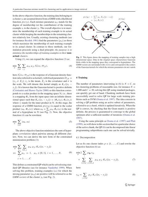
A particular Gaussian mixture model for clustering and its application to image retrievalIn the above objective function, the training data belonging toaclustery l are assumed drawn from a GMM with a likelihoodfunction p(x|y l ). Each mixture parameter µ il stands for thedegree of membership (or the contribution) of the trainingexample x i to the cluster y l . The overall objective is to maximizethe membership of each training example to its actualcluster while keeping the memberships to the remaining clustersrelatively low. Usually, existing clustering methods (seefor instance Bezdek 1981) find the parameters {µ il } as thosewhich maximize the membership of each training exampleto its actual cluster. In contrast to these methods, our formulationproceeds using a dual principle; the purpose is tominimize the memberships of training examples to their nonactualclusters.Using (1), we can expand the objective function (3)as:minµ∑ ∑µ ik µ jl N l (x i ; Θ j|l ), (4)k̸=li, jhere N l (x i ; Θ j|k ) is the response of a Gaussian density function(also referred to as kernel), with fixed parameters Θ j|k ={x j ,σ Σ j }; x j is the mean, Σ j is the covariance and σ isthe scale. We will denote this kernel simply as K σ (‖x i −x j ‖). It is known that the Gaussian kernel is positive definite(Cristianini and Shawe-Taylor 2000) so this function correspondsto a scalar product in the mapping space H, i.e., thereis a mapping Φ σ from the input space into an infinite dimensionalspace such that K σ (‖x i − x j ‖) =〈Φ σ (x i ), Φ σ (x j )〉where 〈〉 stands for the inner product in H. At this stage, theresponse of a GMM function p(x|y k ) is equal to the scalarproduct 〈ω k ,Φ σ (x)〉 where ω k = ∑ i µ ik Φ σ (x i ) is the normalof a hyperplane in H (see Fig. 2). Now, the objectivefunction (4) can be rewritten:minµ∑〈ω k ,ω l 〉 (5)k̸=lThe above objective function minimizes the sum of hyperplanecorrelations taken pairwise among all different clusters.Now, we can derive the new form of the constrainedminimization problem (3):minµs.t.∑k,i∑l̸=k, jµ ik µ jl K σ (‖x i − x j ‖)∑µ ic = 1, µ ic ∈[0, 1], i = 1,...,N,ic = 1,...,CThis defines a constrained QP which can be solved using standardQP libraries (see for instance Vanderbei 1999). Whensolving this problem, training examples {x i } for which themixing parameter {µ ik } are positive will be referred to as theGMM vectors of the cluster y k (see Fig. 2).(6)p(x|y 1 ) = ∑ Niµ i1 K σ (‖x − x i ‖)= 〈ω 1 ,Φ σ (x)〉w 1w 2p(x|y 2 )Fig. 2 This figure shows the mapping of training samples into a highdimensional space. Data in the original space characterizes Gaussianblobs while in the mapping space they correspond to hyperplanes. TheGMM vectors are surrounded with circles and correspond to the centersof the Gaussian kernels for which the mixture parameters do not vanish4 TrainingThe number of parameters intervening in (6) isN × C, sofor clustering problems of reasonable size, for instance N =1.000 and C = 20, solving this QP, using standard packages,can quickly get out of hand. Chunking methods have beensuccessfully used to solve QP for large scale training problemssuch as SVM (Osuna et al. 1997). The idea consists insolving a QP problem using an active subset of parameters,referred to as a chunk, which is updated iteratively. When theQP is convex, by checking that the Gram matrix is positivedefinite, the process is guaranteed to converge to the globaloptimum after a sufficient number of iterations (Osuna et al.1997).Using the same principle as Osuna et al. (1997) and Platt(1999), we will show in this section that for a particular choiceof the active chunk, the QP (6) can be decomposed into linearprogramming subproblems each one can be solved trivially.4.1 DecompositionLet us fix one cluster index p ∈{1,...,C} and rewrite theobjective function (6)as:min 2 ∑ µi+ ∑here:i,k̸=pc ip = ∑j,l̸=pµ ip c ip∑j,l̸=k,pµ ik µ jl K σ (‖x i − x j ‖), (7)µ jl K σ (‖x i − x j ‖) (8)123