A particular Gaussian mixture model for clustering and its ...

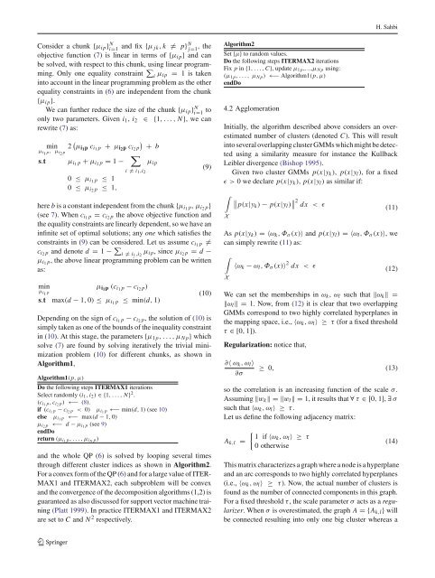
H. SahbiConsider a chunk {µ ip }i=1 N and fix {µ jk, k ̸= p} N j=1 ,theobjective function (7) is linear in terms of {µ ip } and canbe solved, with respect to this chunk, using linear programming.Only one equality constraint ∑ i µ ip = 1 is takeninto account in the linear programming problem as the otherequality constraints in (6) are independent from the chunk{µ ip }.We can further reduce the size of the chunk {µ ip }i=1 N toonly two parameters. Given i 1 , i 2 ∈ {1,...,N}, we canrewrite (7) as:min 2 ( µ i1 p c i1 p + µ i2 p c i2 p)+ bµ i1 p, µ i2 ps.t µ i1 p + µ i2 p = 1 − ∑µ ipi ̸= i 1 ,i 20 ≤ µ i1 p ≤ 10 ≤ µ i2 p ≤ 1,here b is a constant independent from the chunk {µ i1 p,µ i2 p}(see 7). When c i1 p = c i2 p the above objective function andthe equality constraints are linearly dependent, so we have aninfinite set of optimal solutions; any one which satisfies theconstraints in (9) can be considered. Let us assume c i1 p ̸=c i2 p and denote d = 1 − ∑ i ̸= i 1 ,i 2µ ip , since µ i2 p = d −µ i1 p, the above linear programming problem can be writtenas:minµ i1 p (c i1 p − c i2 p)µ i1 ps.t max(d − 1, 0) ≤ µ i1 p ≤ min(d, 1)(9)(10)Depending on the sign of c i1 p − c i2 p, the solution of (10) issimply taken as one of the bounds of the inequality constraintin (10). At this stage, the parameters {µ 1p ,...,µ Np } whichsolve (7) are found by solving iteratively the trivial minimizationproblem (10) for different chunks, as shown inAlgorithm1,Algorithm1(p,µ)Do the following steps ITERMAX1 iterationsSelect randomly (i 1 , i 2 ) ∈{1,...,N} 2 .(c i1 p, c i2 p) ←− (8).if (c i1 p − c i2 p < 0) µ i1 p ←− min(d, 1) (see 10)else µ i1 p ←− max(d − 1, 0)µ i2 p ←− d − µ i1 p (see 9)endDoreturn (µ i1 p,...,µ iN p)and the whole QP (6) is solved by looping several timesthrough different cluster indices as shown in Algorithm2.For a convex form of the QP (6) and for a large value of ITER-MAX1 and ITERMAX2, each subproblem will be convexand the convergence of the decomposition algorithms (1,2) isguaranteed as also discussed for support vector machine training(Platt 1999). In practice ITERMAX1 and ITERMAX2are set to C and N 2 respectively.Algorithm2Set {µ} to random values.Do the following steps ITERMAX2 iterationsFix p in {1,...,C}, update µ 1p ,…,µ Np using:(µ 1p ,..., µ Np ) ←− Algorithm1(p,µ)endDo4.2 AgglomerationInitially, the algorithm described above considers an overestimatednumber of clusters (denoted C). This will resultinto several overlapping cluster GMMs which might be detectedusing a similarity measure for instance the KullbackLeibler divergence (Bishop 1995).Given two cluster GMMs p(x|y k ), p(x|y l ),forafixedɛ>0 we declare p(x|y k ), p(x|y l ) as similar if:∫X∥ p(x|yk ) − p(x|y l ) ∥ ∥ 2 dx < ɛ(11)As p(x|y k ) =〈ω k ,Φ σ (x)〉 and p(x|y l ) =〈ω l ,Φ σ (x)〉, wecan simply rewrite (11) as:∫X〈ω k − ω l ,Φ σ (x)〉 2 dx < ɛ(12)We can set the memberships in ω k , ω l such that ‖ω k ‖=‖ω l ‖=1. Now, from (12) it is clear that two overlappingGMMs correspond to two highly correlated hyperplanes inthe mapping space, i.e., 〈ω k ,ω l 〉 ≥ τ (for a fixed thresholdτ ∈[0, 1]).Regularization: notice that,∂〈 ω k ,ω l 〉∂σ≥ 0, (13)so the correlation is an increasing function of the scale σ .Assuming ‖w k ‖=‖w l ‖=1, it results that ∀ τ ∈[0, 1], ∃ σsuch that 〈ω k ,ω l 〉 ≥ τ.Let us define the following adjacency matrix:A k,l ={ 1 if〈ωk ,ω l 〉 ≥ τ0 otherwise(14)This matrix characterizes a graph where a node is a hyperplaneand an arc corresponds to two highly correlated hyperplanes(i.e., 〈ω k ,ω l 〉 ≥ τ). Now, the actual number of clusters isfound as the number of connected components in this graph.For a fixed threshold τ, the scale parameter σ acts as a regularizer.When σ is overestimated, the graph A ={A k,l } willbe connected resulting into only one big cluster whereas a123